VIO SLAM
IMU
Components
| Components | Measurements | DoF | Description |
|---|---|---|---|
| accelerometer | \(a_b = [a_{bx}, a_{by}, a_{bz}]^T\) | 3 | acceleration (together with gravity) in the sensor body frame |
| gyroscope | \(\omega_b = [\omega_{bx}, \omega_{by}, \omega_{bz}]^T\) | 3 | angular velocity in the sensor body frame |
Properties
- High sampling rate (on the order of hundreds of samples per second)
- Accurate in a short time
- Suffering from drift in a long time range
- Accelerometer and gyroscope can be biased, which means that their measurement errors are not zero-mean (零偏). The bias can vary as time goes. We denote the biases of the accelerometer and gyroscope measurements as \(b^a\) and \(b^g\) respectively.
Model
At time \(t\),
\[\begin{split} \omega_b(t) &= \bar{\omega}_b(t) + b^g(t) + n^g(t), \\ a_b(t) &= R_{wb}(t)^T (\bar{a}_w(t) - g_w) + b^a(t) + n^a(t). \end{split}\]- \(\bar{\omega}\) and \(\bar{a}\) are the true rotational velocity and acceleration in contrast to the noisy measurements \(\omega\) and \(a\).
- \(n^g(t)\) and \(n^a(t)\) are Gaussian noise of the gyroscope and acceleration measurements. Please note that the bias terms and the noise terms are all expressed in the body frame of frame t.
- \(R_{wb}(t)\) is the rotation which rotates a point from the body frame into the world frame at time \(t\).
- \(g_w\) is the gravity acceleration vector in the world frame.
Inertial odometry
Inertial odometry aims at estimating the state of IMU, which is denoted as \(x(t) = [R_{wb}(t), p_w(t), v_w(t)]^T\). \(p_w(t)\) and \(v_w(t)\) are the position and velocity of IMU in the world frame respectively.
\[\begin{split} \frac{d R_{wb}(t)}{dt} &= R_{wb}(t) \frac{d \Delta R_b(t)}{dt} = R_{wb}(t) \bar{\omega}_b(t), \\ \frac{d v_w(t)}{dt} &= \bar{a}_w(t), \\ \frac{d p_w(t)}{dt} &= v_w(t). \end{split}\]- \(\Delta R_b(t)\) is the infinitestimal rotation from time \(t + \Delta t\) to time \(t\) in the body frame.
The update step of the IMU state can be expressed as
\[\begin{split} R_{wb}(t + \Delta t) &= R_{wb}(t) exp( \bar{\omega}_b(t) \Delta t ) \\ &= R_{wb}(t) exp( (\omega_b(t) - b^g(t) - n^g(t)) \Delta t ), \\ v_w(t + \Delta t) &= v_w(t) + \bar{a}_w(t) \Delta t \\ &= v_w(t) + g_w \Delta t + R_{wb}(t) (a_b(t) - b^a(t) - n^a(t)) \Delta t, \\ p_w(t + \Delta t) &= p_w(t) + v_w(t) \Delta t + \frac{1}{2} \bar{a}_w(t) \Delta t^2 \\ &= p_w(t) + v_w(t) \Delta t + \frac{1}{2} g_w \Delta t^2 + \frac{1}{2} R_{wb}(t) (a_b(t) - b^a(t) - n^a(t)) \Delta t^2. \end{split}\]- Here we use lie algebra for the representation of rotation velocity.
- Note that we assume a constant rotation \(R_{wb}(t)\) during the short sampling period \(\Delta t\).
- Computing \(R_{wb}(t + \Delta t)\) is straightforward just by intergating the rotational velocity, while computing \(p_w(t + \Delta t)\) is cumbersome because not only does it rely on the double integration of the acceleration measurements but also the estimation of orientation \(R_{wb}(t)\).
Equivalently, we can express the equations above in discrete time steps of length \(\Delta t\). Subscripts are omitted for each of notation.
\[\begin{split} R_{i+1} &= R_i exp( \bar{\omega}_i \Delta t) \\ &= R_i exp( (\omega_i - b^g_i - n^g_i) \Delta t), \\ v_{i+1} &= v_i + \bar{a}_i \Delta t \\ &= v_i + g \Delta t + R_i (a_i - b^a_i - n^a_i) \Delta t, \\ p_{i+1} &= p_i + v_i \Delta t + \frac{1}{2} \bar{a}_i \Delta t^2 \\ &= p_i + v_i \Delta t + \frac{1}{2} g \Delta t^2 + \frac{1}{2} R_i (a_i - b^a_i - n^a_i) \Delta t^2. \end{split}\]Rather than looking at a discrete step \((i, i+1)\), we can pre-integrate the state dynamics in longer intervals, e.g., \((i, j)\).
\[\begin{split} R_j &= R_i exp( \sum_{k=i}^{j-1} \bar{\omega}_k \Delta t) \\ &= R_i exp( \sum_{k=i}^{j-1} (\omega_k - b^g_k - n^g_k) \Delta t) \\ &= R_i \prod_{k=i}^{j-1} exp( (\omega_k - b^g_k - n^g_k) \Delta t) \\ v_j &= v_i + \sum_{k=i}^{j-1} \bar{a}_k \Delta t \\ &= v_i + (j-i) g \Delta t + \sum_{k=i}^{j-1} R_k (a_k - b^a_k - n^a_k) \Delta t, \\ p_j &= p_i + \sum_{k=i}^{j-1} v_k \Delta t + \frac{1}{2} \sum_{k=i}^{j-1} \bar{a}_k \Delta t^2 \\ &= p_i + \sum_{k=i}^{j-1} v_k \Delta t + (j-i) \frac{1}{2} g \Delta t^2 + \sum_{k=i}^{j-1} \frac{1}{2} R_k (a_k - b^a_k - n^a_k) \Delta t^2. \end{split}\]Pre-integration (see [2] for reference)
The problem of the equations above is that they require the knowledge of the initial state at time \(i\), i.e., \(x_i = [R_i, p_i, v_i]^T\). However, in some cases, we have no idea of the initial state. Therefore, pre-integration is usually adopted to integrate the measurements in the body frame of the last state. Then, once the initial state is available, the subsequent states can be brought into the world frame by simple addition or multiplication with the pre-integration values.
Below, we ignore the addition terms concerning \(g\) for simplicity, since they are constant for a fixed length of interval. The pre-integration is written as below.
\[\begin{split} \Delta R_{ij} &= R_i^T R_j = \prod_{k=i}^{j-1} exp( (\omega_k - b^g_k - n^g_k) \Delta t) \\ \Delta v_{ij} &= R_i^T(v_j - v_i) = \sum_{k=i}^{j-1} \Delta R_{ik} (a_k - b^a_k - n^a_k) \Delta t, \\ \Delta p_{ij} &= R_i^T (p_j - p_i - (j-i) v_i )= \sum_{k=i}^{j-1} \Delta v_{ik} \Delta t + \sum_{k=i}^{j-1} \frac{1}{2} \Delta R_{ik} (a_k - b^a_k - n^a_k) \Delta t^2. \end{split}\]- Here \(\Delta R_{ij}\), \(\Delta v_{ij}\) and \(\Delta p_{ij}\) represent the pre-integrated measurements derived from the raw IMU measurements \(a\) and \(\omega\), which relate the states of keyframes i and j.
- \(\Delta R_{ij}\) denotes the physical relative rotation that brings a point in the j-th body frame into the i-th body frame.
- But \(\Delta v_{ij}\) and \(\Delta p_{ij}\) do not correspond to the true physical change in the velocity and position.
- Currently, the right hand side of the above equations are independent of the initial state \(x_i = [R_i, p_i, v_i]^T\), and can be obtained solely from the measurements.
- Once \([R_i, p_i, v_i]^T\) and \([\Delta R_{ij}, \Delta p_{ij}, \Delta v_{ij}]^T\) are known, the state \([R_j, p_j, v_j]^T\) can be easily computed.
Noise propagation
The pre-integrated measurements above involve the raw measurement noise. It is better to isolate the noise terms from the pre-integated quantities, so that likelihood models can be easily applied. Therefore, below the noise modeling of the pre-integrated measurements are derived in a way of simple addition or multication with the noise-free terms.
Rotation noise
\[\begin{split} \Delta R_{ij} &= \prod_{k=i}^{j-1} exp( (\omega_k - b^g_k) \Delta t - n^g_k \Delta t) \\ &= \prod_{k=i}^{j-1} exp( (\omega_k - b^g_k) \Delta t) exp( - J_k n^g_k \Delta t) \\ &= \Delta\tilde{R}_{ij} \prod_{k=i}^{j-1} exp (-\Delta \tilde{R}_{k+1,j}^T J_k n_k^g \Delta t) \\ &= \Delta\tilde{R}_{ij} exp(-\delta \Phi_{ij}) \end{split}\]- \(\Delta\tilde{R}_{ij}\) is the noise-free rotation from frame j to frame i.
- The rotation noise \(\delta \Phi_{ij} = -log( \prod_{k=i}^{j-1} exp (-\Delta \tilde{R}_{k+1,j}^T J_k n_k^g \Delta t) )\) depends on the raw measurement noise \(n_k^g\). Since \(n_k^g\) is small noise, we can approximately get \(\delta \Phi_{ij} \approx \sum_{k=i}^{j-1} \Delta \tilde{R}_{k+1,j}^T J_k n_k^g \Delta t\). In this way, \(\delta \Phi_{ij}\) is the linear combination of \(n_k^g\) and is thus zero-mean and Gaussian.
- \(J_k\) is the right Jacobian of SO(3) and \(exp(\Phi + \delta \Phi) \approx exp(\Phi) exp(J(\Phi) \delta\Phi)\) is the first-order approximation.
- The third line above is derived based on the formula \(exp(\Phi)R = R exp(R^T \phi)\), so that \(R_1 exp(\Phi_1) R_2 exp(\Phi_2) = R_1 R_2 exp(R_2^T \Phi_1) exp(\Phi_2)\). By a series of such operations, we can move the noise terms to the end.
Velocity noise
\[\begin{split} \Delta v_{ij} & \approx \sum_{k=i}^{j-1} \Delta \tilde{R}_{ik} (I - \delta \Phi_{ik}^\wedge) (a_k - b^a_k - n^a_k) \Delta t \\ &= \sum_{k=i}^{j-1} \Delta \tilde{R}_{ik} (a_k - b^a_k) \Delta t - \Delta \tilde{R}_{ik} \delta \Phi_{ik}^\wedge (a_k - b^a_k) \Delta t - \Delta\tilde{R}_{ik} n^a_k \Delta t \\ &= \Delta \tilde{v}_{ij} + \sum_{k=i}^{j-1} (\Delta \tilde{R}_{ik} (a_k - b^a_k)^\wedge \delta \Phi_{ik} \Delta t - \Delta\tilde{R}_{ik} n^a_k \Delta t) \\ &= \Delta \tilde{v}_{ij} - \delta v_{ij} \end{split}\]- \((a_k - b^a_k) \Delta t\) is the noise-free velocity change in frame k, and \(\Delta \tilde{R}_{ik} (a_k - b^a_k) \Delta t\) transforms the change into frame i. Therefore, \(\Delta \tilde{v}_{ij} = \sum_{k=i}^{j-1} \Delta \tilde{R}_{ik} (a_k - b^a_k) \Delta t\) accumutates the velocity changes in later steps in the local frame i.
- The velocity noise \(\delta v_{ij} = - \sum_{k=i}^{j-1} (\Delta \tilde{R}_{ik} (a_k - b^a_k)^\wedge \delta \Phi_{ik} \Delta t - \Delta\tilde{R}_{ik} n^a_k \Delta t)\) is linear with both integrated rotational noise \(\delta \Phi_{ik}\) and the acceleration noise \(n^a_k\), and is thus zero-mean and Gaussian.
- The higher-order noise terms such as \(\Phi_{ik} * n^a_k\) are neglected.
Position noise
\[\begin{split} \Delta p_{ij} &= \sum_{k=i}^{j-1} (\Delta \tilde{v}_{ik} - \delta v_{ik} )\Delta t + \frac{1}{2} \Delta \tilde{R}_{ik} (I - \delta \Phi_{ik}^\wedge) (a_k - b^a_k) \Delta t^2 - \frac{1}{2} \Delta \tilde{R}_{ik} n_k^a \Delta t^2 \\ &= \sum_{k=i}^{j-1} (\Delta \tilde{v}_{ik} \Delta t + \frac{1}{2} \Delta \tilde{R}_{ik} (a_k - b^a_k) \Delta t^2 ) \\ &- \sum_{k=i}^{j-1} (\delta v_{ik} \Delta t - \frac{1}{2} \Delta\tilde{R}_{ik} (a_k - b^a_k)^\wedge \delta \Phi_{ik} \Delta t^2 + \frac{1}{2} \Delta \tilde{R}_{ik} n_k^a \Delta t^2) \\ &= \Delta \tilde{p}_{ij} + \delta p_{ij} \end{split}\]- \(\Delta \tilde{p}_{ij}\) is the noise-free accumulated translation in the local frame i.
- \(\delta p_{ij}\) is linear with the pre-integrated rotation noise \(\delta \Phi_{ik}\), the pre-integrated velocity noise \(\delta v_{ik}\) and the acceleration noise \(n_k^a\), and is thus zero-mean and Gaussian.
Update
If we consider the inertial dynamics as a recurrent process, one of the important steps is to update the inherent states as new measurements are collected over time. Here, the states include the pre-integrated noise-free rotation \(\Delta\tilde{R}_{ij}\), velocity \(\Delta \tilde{v}_{ij}\), position \(\Delta \tilde{p}_{ij}\), covariances of rotation noise \(\delta \Phi_{ij}\), velocity noise \(\delta v_{ij}\) and position noise \(\delta p_{ij}\).
The transition of the aforementioned states can be computed as follows.
\[\begin{split} \Delta\tilde{R}_{ij} &= \Delta\tilde{R}_{i,j-1} exp( (\omega_j - b^g_j) \Delta t), \\ \Delta \tilde{v}_{ij} &= \Delta \tilde{v}_{i,j-1} + \Delta\tilde{R}_{i,j-1} (a_{j-1} - b^a_{j-1}) \Delta t, \\ \Delta \tilde{p}_{ij} &= \Delta \tilde{p}_{i,j-1} + \Delta \tilde{v}_{i,j-1} \Delta t + \frac{1}{2} \Delta\tilde{R}_{i,j-1} (a_{j-1} - b^a_{j-1}) \Delta t^2. \end{split}\]The transition of the covariances of rotation noise \(\delta \Phi_{ij}\), velocity noise \(\delta v_{ij}\) and position noise \(\delta p_{ij}\) is a bit more complicated because the velocity noise \(\delta v_{ij}\) depends on the rotation noise \(\delta \Phi_{ij}\), and the position noise \(\delta p_{ij}\) depends on both the rotation noise \(\delta \Phi_{ij}\) and the velocity noise \(\delta v_{ij}\).
\[\begin{split}\delta \Phi_{ij} &\approx \sum_{k=i}^{j-1} \Delta \tilde{R}_{k+1,j}^T J_k n_k^g \Delta t \\ &= \sum_{k=i}^{j-2} \Delta \tilde{R}_{k+1,j}^T J_k n_k^g \Delta t + J_{j-1} n_{j-1}^g \Delta t \\ &= \sum_{k=i}^{j-2} (\Delta\tilde{R}_{k+1,j-1} \Delta\tilde{R}_{j-1,j} )^T J_k n_k^g \Delta t + J_{j-1} n_{j-1}^g \Delta t \\ &= \Delta\tilde{R}_{j-1,j}^T \sum_{k=i}^{j-2} \Delta\tilde{R}_{k+1,j-1}^T J_k n_k^g \Delta t + J_{j-1} n_{j-1}^g \Delta t \\ &= \Delta\tilde{R}_{j-1,j}^T \delta \Phi_{i,j-1} + J_{j-1} n_{j-1}^g \Delta t. \\ \delta v_{ij} &= - \sum_{k=i}^{j-1} (\Delta \tilde{R}_{ik} (a_k - b^a_k)^\wedge \delta \Phi_{ik} \Delta t - \Delta\tilde{R}_{ik} n^a_k \Delta t) \\ &= - \sum_{k=i}^{j-2} (\Delta \tilde{R}_{ik} (a_k - b^a_k)^\wedge \delta \Phi_{ik} \Delta t - \Delta\tilde{R}_{ik} n^a_k \Delta t) - \Delta \tilde{R}_{i,j-1} (a_{j-1} - b^a_{j-1})^\wedge \delta \Phi_{i,j-1} \Delta t + \tilde{R}_{i,j-1} n^a_{j-1} \Delta t \\ &= \delta v_{i,j-1} - \Delta \tilde{R}_{i,j-1} (a_{j-1} - b^a_{j-1})^\wedge \delta \Phi_{i,j-1} \Delta t + \Delta\tilde{R}_{i,j-1} n^a_{j-1} \Delta t. \\ \delta p_{ij} &= - \sum_{k=i}^{j-1} (\delta v_{ik} \Delta t - \frac{1}{2} \Delta\tilde{R}_{ik} (a_k - b^a_k)^\wedge \delta \Phi_{ik} \Delta t^2 + \frac{1}{2} \Delta \tilde{R}_{ik} n_k^a \Delta t^2) \\ &= - \sum_{k=i}^{j-2} (\delta v_{ik} \Delta t - \frac{1}{2} \Delta\tilde{R}_{ik} (a_k - b^a_k)^\wedge \delta \Phi_{ik} \Delta t^2 + \frac{1}{2} \Delta \tilde{R}_{ik} n_k^a \Delta t^2) \\ &- (\delta v_{i,j-1} \Delta t - \frac{1}{2} \Delta\tilde{R}_{i,j-1} (a_{j-1} - b^a_{j-1})^\wedge \delta \Phi_{i,j-1} \Delta t^2 + \frac{1}{2} \Delta \tilde{R}_{i,j-1} n_{j-1}^a \Delta t^2) \\ &= \delta p_{i,j-1} - (\delta v_{i,j-1} \Delta t - \frac{1}{2} \Delta\tilde{R}_{i,j-1} (a_{j-1} - b^a_{j-1})^\wedge \delta \Phi_{i,j-1} \Delta t^2 + \frac{1}{2} \Delta \tilde{R}_{i,j-1} n_{j-1}^a \Delta t^2). \end{split}\]Let \(N_{ij} = [\delta \Phi_{ij}^T, \delta v_{ij}^T, \delta p_{ij}^T]^T\), then relationship between \(N_{ij}\) and \(N_{i,j-1}\) can be expressed as
\[N_{ij} = \mathbf{A}_{j-1} N_{i,j-1} + \mathbf{B}_{j-1} n_{j-1}^g + \mathbf{C}_{j-1} n_{j-1}^a.\]In this way, the covariance of noise \(N_{ij}\) can be updated as below:
\[\Sigma_{ij} = \mathbf{A}_{j-1} \Sigma_{i,j-1} \mathbf{A}_{j-1}^T + \mathbf{B}_{j-1} \Sigma_{i,j-1}^g \mathbf{B}_{j-1}^T + \mathbf{C}_{j-1} \Sigma_{i,j-1}^a \mathbf{C}_{j-1}^T,\]where \(\Sigma_{i,j-1}^g\) is the measurement noise covariance of gyroscope and \(\Sigma_{i,j-1}^a\) is the measurement noise covariance of accelerometer.
Visual inertial odometry
Initialization
The initialization is to estimate or calibrate the variables:
- scale (of visual coordinate system),
- gravity direction,
- gyroscope bias and accelerometer bias,
- velocity.
The variables are hard to be solved by one pass. Therefore, they are generally computed sequentially followed by a global optimization.
Gyroscope bias estimation
If we ignore the noise terms in the preintegration formula for rotation, we get
\[\begin{split} \Delta R_{ij} &= \prod_{k=i}^{j-1} exp( (\omega_k - b^g_k) \Delta t) \\ &= \prod_{k=i}^{j-1} exp( \omega_k \Delta t) exp( - J_k b^g_k \Delta t) \\ &= \Delta\hat{R}_{ij} \prod_{k=i}^{j-1} exp (-\Delta \hat{R}_{k+1,j}^T J_k b_k^g \Delta t) \\ &= \Delta\hat{R}_{ij} exp(-\delta \Psi_{ij}), \end{split}\]where \(\delta \Psi_{ij} \approx \sum_{k=i}^{j-1} \Delta \hat{R}_{k+1,j}^T J_k b_k^g \Delta t\) and it can be updated recursively by \(\delta \Psi_{i,j+1} = \Delta\hat{R}_{j+1,j} \delta \Psi_{ij} + J_j b_j^g \Delta t\). \(\Delta\hat{R}_{ij} = \prod_{k=i}^{j-1} exp( \omega_k \Delta t).\)
If we run visual SLAM, we can also get the relative rotation between keyframe i and j as \(\Delta R_{ij} = R_i R_j^T\). In this way, the Gyroscope bias can be estimated by minimizing the loss \(\sum \| (R_i R_j^T)^T \Delta\hat{R}_{ij} exp(-\delta \Psi_{ij}) \|^2\).
Scale and gravity estimation
Let \(p_{cb}\) denote the position of IMU sensor in the camera coordinate frame. The IMU coordinates can be transformed into the camera frame up to an unknown scale \(s\):
\[p_i = s p_i^c + R_c p_{cb},\]where \(p_i^c\) is the coordinates of the camera center of keyframe i.
From above, we have that
\[\begin{split} p_j &= p_i + \sum_{k=i}^{j-1} v_k \Delta t + (j-i) \frac{1}{2} g \Delta t^2 + \sum_{k=i}^{j-1} \frac{1}{2} R_k (a_k - b^a_k - n^a_k) \Delta t^2 \\ &= p_i + v_i \Delta t_{ij} + \frac{1}{2}(j-i)g\Delta t^2 + R_i \Delta p_{ij}.\end{split}\]Substitute \(p_i = s p_i^c + R_c p_{cb}\) into the equation above, we get
\[sp_j = sp_i + v_i \Delta t_{ij} + \frac{1}{2}(j-i)g\Delta t^2 + R_i \Delta p_{ij} + (R_i - R_j)p_{cb}.\]In order to eliminate the variable \(v_i\) to reduce the complexity, we write two consecutive equations for keyframe 1, 2 and 3:
\[\begin{split} sp_2 = sp_1 + v_1 \Delta t_{12} + \frac{1}{2}g\Delta t_{12}^2 + R_1 \Delta p_{12} + (R_1 - R_2)p_{cb}, \\ sp_3 = sp_2 + v_2 \Delta t_{23} + \frac{1}{2}g\Delta t_{23}^2 + R_2 \Delta p_{23} + (R_2 - R_3)p_{cb}. \end{split}\]Multiply \(\Delta t_{23}\) and \(\Delta t_{12}\) with above equation respectively,
\[\begin{split} sp_2 \Delta t_{23} = sp_1 \Delta t_{23} + v_1 \Delta t_{12} \Delta t_{23} + \frac{1}{2}g\Delta t_{12}^2 \Delta t_{23} + R_1 \Delta p_{12} \Delta t_{23} + (R_1 - R_2)p_{cb} \Delta t_{23}, \\ sp_3 \Delta t_{12} = sp_2 \Delta t_{12} + v_2 \Delta t_{23} \Delta t_{12} + \frac{1}{2}g\Delta t_{23}^2 \Delta t_{12} + R_2 \Delta p_{23} \Delta t_{12} + (R_2 - R_3)p_{cb} \Delta t_{12}. \end{split}\]After the substraction, we get
\[\begin{split} &((p_2 - p_1) \Delta t_{23} - (p_3 - p_2) \Delta t_{12})s + \frac{1}{2}(\Delta t_{23}^2 \Delta t_{12} - \Delta t_{12}^2 \Delta t_{23}) g \\ = &\Delta t_{12}\Delta t_{23} (v_1 - v_2) + R_1 \Delta p_{12} \Delta t_{23} - R_2 \Delta p_{23} \Delta t_{12} + (R_1 - R_2) p_{cb} \Delta t_{23} - (R_2 - R_3) p_{cb} \Delta t_{12} \\ =&-\Delta t_{12}\Delta t_{23} R_1 \Delta v_{12} + R_1 \Delta p_{12} \Delta t_{23} - R_2 \Delta p_{23} \Delta t_{12} + (R_1 - R_2) p_{cb} \Delta t_{23} - (R_2 - R_3) p_{cb} \Delta t_{12} \end{split}\]In this way, we get a linear system for the neighboring 3 keyframes. We can stack all the linear equations from all consecutive triple-frames to solve \(s\) and \(g\).
Please note that \(\Delta p_{12}\) and \(\Delta p_{23}\) computed above do not consider the accelerometer bias which is still unknown, because gravity and accelerometer bias are hard to distinguish. Therefore, we first ignore accelerometer bias and estimate the gravity roughly, and then estimate accelerometer bias and refine gravity in the next stage.
Accelerometer bias estimation
The gravity vector computed in the last stage is in the world coordinate system. Let’s denote it as \(g_W\). If we consider a coordinate system which defines the gravity as \(G g_I = G [0, 0, -1]^T\) (\(G\) is the gravity magnitude), we have \(g_W = G R_{WI} g_I\), where \(R_{WI}\) is the rotation from \(g_I\) to \(g_W\) and it only has rotations around x and y axes.
Since the gravity direction computed in the last stage is not perfect, we can add a small rotation into \(g_W\) as
\[\begin{split} g_W &= G R_{WI} Exp(\delta \theta) g_I, \\ &\approx G R_{WI} (I + {\delta \theta}_x) g_I, \\ &\approx G R_{WI} g_I - G R_{WI} {g_I}_x \delta \theta. \end{split}\]where \(\delta \theta = [\delta \theta_x, \delta \theta_y, 0]^T\) only contains rotations around x and y axes.
Since now we consider the accelerometer bias in the pre-integration of position, we have
\[\Delta p_{ij} = \Delta \hat{p}_{ij} - \frac{3}{2} \sum_{k=i}^{j-1} \Delta R_{ik} b^a \Delta t^2.\]Substituting the equations above into
\[sp_j = sp_i + v_i \Delta t_{ij} + \frac{1}{2}(j-i)g\Delta t^2 + R_i \Delta p_{ij} + (R_i - R_j)p_{cb},\]we get the linear equation about \([s, \delta \theta, b_a]^T\) from the three consecutive keyframes in a similar way to the last stage, and refine scale and gravity direction and solve accelerometer bias simultaneously.
Velocity estimation
After scale, gravity, gyroscope and accelerometer bias are all estimated, the velocity of keyframes can be estimated from the equation below.
\[sp_j = sp_i + v_i \Delta t_{ij} + \frac{1}{2}(j-i)g\Delta t^2 + R_i \Delta p_{ij} + (R_i - R_j)p_{cb}.\]Keyframe selection
VIO-mono
- The average parallax of tracked features between current frame and the latest keyframe is beyond a certain threshold. To avoid rotation-only parallax, rotation compensation via IMU integration is used.
- The number of tracked features goes below a certain threshold.
ORB-SLAM (Surval of the fittest strategy)
- Time from last keyframe > 0.5s.
- Frames from last keyframe > 30.
- The number of tracked features goes below a certain threshold.
- Delete redundant keyframes whose 90% of the map points have been seen in at least other three keyframes.
Measurement/keyframe culling
In order to reduce the computational cost for real-time performance, [6] proposed a measurement and keyframe culling approach to reduce the redundancy of a pose graph based on the information matrix (or the Hessian matrix).
For a track with projections indexed by \(j\), bundle adjustment builds the information matrix \(V\) as
\[V = \sum_j V_j = \sum_j J_j^T \Sigma_j^{-1} J_j,\]where \(J_j \in R_{2x3}\) is the Jacobian matrix and \(\Sigma_j^{-1}\) is the measurement noise. The determinant of \(V\) is a metric corresponding to the amount of information constraining the position of the point given camera poses. For each projection, we consider the metric \(m_j = det(V) - det(V-V_j)\) as the information loss after the measurement is removed. A low value indicates the measurement is redundant and can be removed (e.g., the measurement is from a redundant viewpoint, the measurement noise is large, or it may be an outlier).
The measurements will also give votes to the keyframes based on the metric \(m_j\). The keyframe with the lowest score can be removed because its measurements are the most redundant.
Pose tracking
Since SLAM runs in an incremental fashion, pose tracking is a recursive step to build the pose of the next frame and the associated new tracks and projections repeatedly.
[4] “Once the camera pose is predicted, the map points in the local map are projected and matched with keypoints on the frame. We then optimize current frame j by minimizing the feature reprojection error of all matched points and an IMU error term.”
It may also be responsible for deciding if the current frame is a keyframe. Once a new keyframe is inserted, local optimization is triggered to optimize the states (poses, velocities and IMU biases) of the last N keyframes.
Relocalization
-
Loop detection. Use DBoW2 to retrieve top-k image candidates for each keyframe. Then for each candidate, perform geometric verification (e.g. computing fundamental matrix or PnP or computing euclidean/similarity transform) to eliminate false-positive retrievals.
-
Loop closure. Pose-graph optimization (or called essential graph optimization by ORB-SLAM) takes into account loop edges, sequential edges (between neighboring frames) and covibility edges (between frames with more than 100 covisible tracks).
Note: For VIO Slam, “the visual-inertial setup renders roll and pitch angles fully observable, the accumulated drift only occurs in four degrees of freedom (x, y, z and yaw angle). To this end, we ignore estimating the drift-free roll and pitch states, and only perform 4-DOF pose graph optimization.” Here “roll and pitch angles fully observable” means that we can compute the absolute pitch and roll angles of IMU in the world frame based on the gravity direction in the IMU body frame. See [5] for details.
Optimization
The factor graph of visual inertial optimization using both visual and inertial measurements is shown as below.
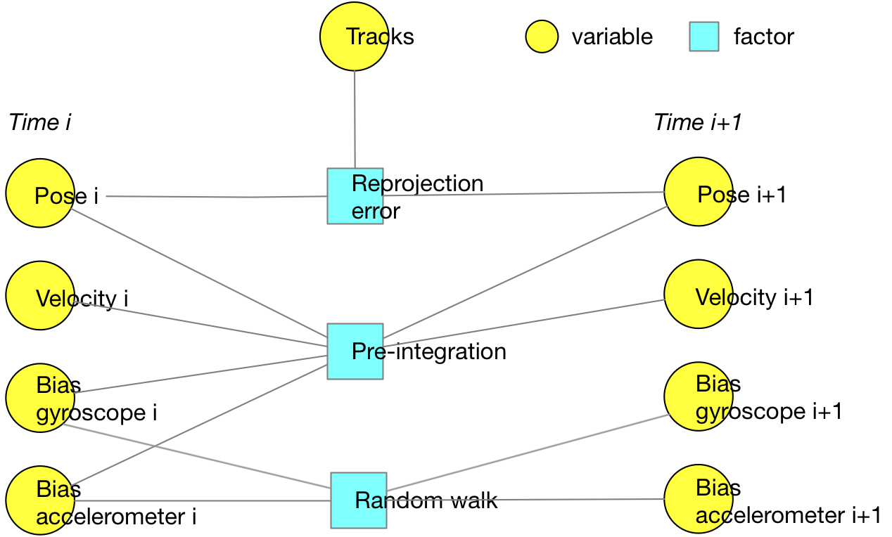
Since the three types of factors arise from different types of measurements, i.e., the visual measurements, the pre-integrated IMU measurements and random walk measurements for bias. In order to sum up the errors from the factors, an information matrix must be multiplied with each error term as a way of weighting (e.g., \(e^T \Sigma e\)).
-
For the visual measurements, the information matrix is inversely proportional to the feature scales.
-
For the pre-integrated IMU measurements, the information matrix is the inverse of the covariance of the rotation, velocity and position noise introduced above.
-
For the random walk measurements for bias, the information matrix is inversely proportional to the white noise covariance whose magnitude grows as time lasts. (See the explanation below.)
The output of a gyro (same for accelerometer) will be perturbed by some thermo-mechanical noise which fluctuates at a rate much greater than the sampling rate of the sensor. As a result the samples obtained from the sensor are perturbed by a white noise sequence, which is simply a sequence of zero-mean uncorrelated random variables. In this case each random variable is identically distributed and has a finite variance.
Multi-threading
In ORB-SLAM, there are three threads working in parallel:
- tracking thread: process the IMU and visual sensor measurements (preintegration, feature detection and matching), localize the current frame, determine if it is a keyframe, relocalize if tracking lost,
- local mapping thread: once a keyframe is added, optimize the active map in a local window,
- loop closure thread: detect loops and run loop closure optimization (pose graph optimization + full bundle).
The active map is locked when it is to be changed by any threads.
Reference
[1] IMU Preintegration on Manifold for Efficient Visual-Inertial Maximum-a-Posteriori Estimation (* Note: there are errors with Eqs. 26.)
[2] On-Manifold Preintegration for Real-Time Visual-Inertial Odometry (* Note: journal version of [1], recommended.)
[3] VINS-Mono: A Robust and Versatile Monocular Visual-Inertial State Estimator
[4] Visual-Inertial Monocular SLAM with Map Reuse
[5] Inertial Measurement Units (Stanford University)
[6] Parallel Tracking and Mapping on a Camera Phone