All You Need to Know About Diffusion Model

• The Essence of Diffusion Model
• The Scheduler
• Sampling
• Learn the Mapping
• Probabilistic Modeling
• Loss Functions
• Training Algorithm
• Reference

The Essence of Diffusion Model

In diffusion model, there is a pre-defined sequence of data samples which are the interpolations between clean data (e.g., \(x_0\)) and pure gaussian noise (e.g., \(x_T\)). The forward path going from clean data to pure gaussian noise is called diffusion process, while the backward direction is called generation process.

The diffusion process adds gaussian noise into data step by step according to some pre-defined scheduler. Therefore, if \(x_0\) is given, all the intermediate data points (or their distributions) are known. Reversally, the objective of generation process is to predict the data points (or their distributions) of previous steps (e.g., \(x_{t-1}\)) from the later steps (e.g., \(x_t\)) until clean data is recovered.

Since both the diffusion and generation processes are stochastic, the training and inference (it’s called sampling in the algorithm chart below) of diffusion models use samples from distributions to train the network. In this way, the inference results are always random due to the random sampling process.

The Scheduler

The definition of the intermediate data points between original data \(x_0\) and pure gaussian noise \(x_T\) in the forward process is totally manual but can be interesting. We call it “scheduler” as we intentionally determine how many steps we have in the forward process and how much noise should be added to the intermediate data samples, i.e.,

where \(\alpha_t\) are all pre-defined. (Basically \(x_t\) is the interpolation between the original data \(x_0\) and gaussian noise.)

The scheduling choice is a trade-off problem because we want to use more steps to reduce the level of noise added in each step so that denoising is feasible, while, on the other hand, we hope the step number to be smaller so that generative process can be efficient.

Sampling

diffusion process from a data sample to pure gaussian noise, where gaussian noise is added intentionally step by step. Since the gaussian noise of each step is pre-defined, we know the distribution of all the intermediate data in each step which has noise of different levels added into the origial data.

Reversally, if we can remove the noise for each intermediate noisy data sample by predicting the noise injected in each step, we can achieve denoising back to the original noise-free data. So after the forward diffusion process has been determined, the remaining work is to train a regression network that is able to predict the noise of step \(t\) that was added to \(x_{t-1}\) to form \(x_t\). Since we have the ground truth of \(x_t\) derived from the diffusion process, the training is feasible.

But the heuristic part of diffusion model is how to determine the forward diffusion process (or called sampling process). For DDPM, we predefine how many steps to use and the magnitude of gaussian noise for each step, which play an important role in the performance of the trained diffusion model. For DDIM, ……

Learn the Mapping

Diffusion model is actually learning the mapping between an unknown data distribution and a known distribution, i.e., \(\mathbf{T}: R^d \leftrightarrow R^d\). The distributions have the same dimensions \(d\). With a known distribution, we can generate infinite samples from it easily, and map them back to the unknown distribution which is more interesting to us, for example, the human language distribution, the image set distribution, or even the distribution of the universe.

Gaussian Is an Option. In practice, we can choose any known distributions we like to learn the mapping. But in general, standard Gaussian distribution is used, because it is easy to understand and simple to implement. Theoretically, it is also possible to map any distributions to a Gaussian distribution given a sufficiently large number of diffusion steps.

Learn the mapping in reduced dimension. In terms of the data space where the mapping is learned, one option is to keep the original high-dimensional data space, for example, millions of dimensions for a high-resolution image. The other option is to transform the original data space into a low-dimensional latent space and learn the mapping in the latent space, which is exactly what StableDiffusion proposed to do. Generally speaking, the dimension is the higher the better, because higher dimension means larger capacity for capturing a complex data distribution. However, many of the data distributions are highly correlated across dimensions and therefore redundant. It is always beneficial to apply a PCA-like transformation to compress the data dimensionality. At the same time, it has the benefit of only keeping the high-level semantic information in the latent space. Therefore, choosing the dimension of the latent space is non-heuristics. It depends on how much essential information we want to capture in the latent space with the lowest dimensionality. Additionally, reducing the dimension to a latent space makes it easier to train the mapping function and more efficient to run sampling.

Probabilistic Modeling

Knowing the mapping from a data distribution of interest, e.g., an image set, to a Gaussian distribution is useless, while the reverse is what we want. The reverse mapping from a sample in Gaussian distribution (e.g., \(y \in N(0,\Sigma)\)) to a sample in an image set is not deterministic, but probabilistic. Given a Gaussian sample \(y\), learning the reverse mapping is to uncover the conditional probability \(p(x\|y)\), where \(x\) is a sample in image set. Mathematically, knowing \(p(x\|y)\) is equivalent to knowing \(p(x, y)\), since \(p(x, y) = p(y) p(x\|y)\) and \(p(y)\) is already known.

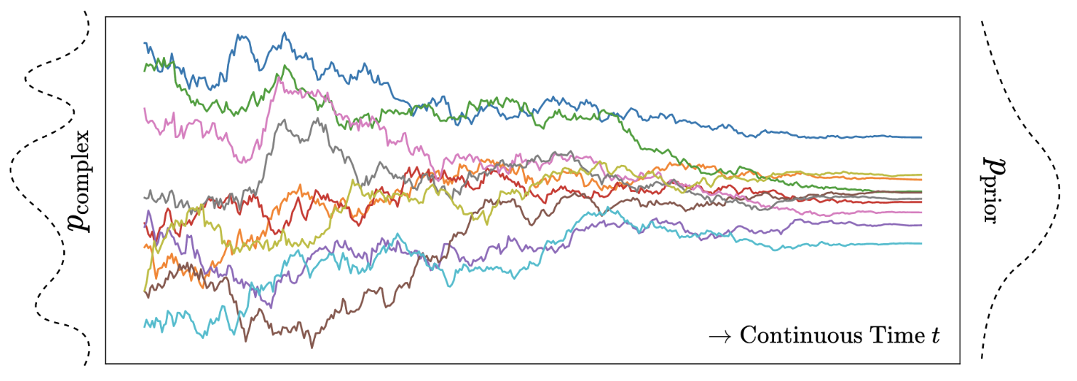
Hard Things in Small Steps. The transform from any distribution to a Gaussian distribution can be easily modelled as a diffusion process as in Physics world, where noise is added into the data gradually and releatedly with a self-defined Markov chain. The basic logic is that every distribution can be seen as piecewise Gaussian. Similarly, we can also learn the reverse process gradually in many small steps, as learning a single-step mapping \(p(x\|y)\) is almost intractable when the distribution of \(x\) is complicated.

Once we decompose the mapping into a bunch of small steps, we get the hidden variables in the same number as the steps. Let’s denote the variable of the image set distribution as \(x_0\), and the variable of the final Gaussian distribution as \(x_T\). We have a number of \(T-1\) intemediate hidden variables \(x_1, x_2, ..., x_{T-1}\) transitioning from \(x_0\) to \(x_T\). The number of the steps depend on how far away the original distribution of \(x_0\) is from a Gaussian distribution.

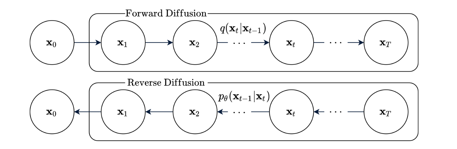
The benefit of these hidden variables is that they make it easier to learning mapping between two very different distributions. On the one hand, it is more effortless to train small substeps than a single huge step, because the regularization of the hidden variable distributions can make the optimization more stable. On the other hand, if one step fails to learn well, the other steps can compensate for that and give an overall good performance. This is how we get the figure below:

Forward Diffusion In the forward diffusion process, the hidden variable \(x_t\) is conditioned only on the last hidden variable \(x_{t-1}\) due to Markov property, i.e., \(p(x_t \| x_{t-1}, ..., x_0) = p(x_t \| x_{t-1})\). Particuarly, we use Gaussian diffusion process here. So we have \(x_t \sim \mathbf{N}(\sqrt{1-\beta_t} x_{t-1}, \beta_t \mathbf{I})\), where \(\beta_t\) is a pre-defined constants reflecting the noise quantity. In practice, we let \(\beta_t\) grow as \(t\) increases, which means we add more noise in the later diffusion steps than in the early steps. It can be interpreted as filtering out higher frequency signals prior to lower frequency signals. In the reserval process, it is natural that lower frequency data is generated earlier than higher frequency data, because lower frequency data generally represents more prenominant features.

After a large finite number of \(T\) steps, we will have \(x_T \sim \mathbf{N}(\mathbf{0}, \mathbf{I})\). With the forward diffusion process defined, we can express the distribution of the diffused sample at any timestamp \(t\) in closed form:

where \(\alpha_t = 1 - \beta_t\) and \(\hat{\alpha_t} = \prod_{s=1}^t \alpha_s\).

Reverse Diffusion Although the forward conditionals \(p(x_t \| x_{t-1})\) are clearly predefined, the reverse conditionals \(q(x_{t-1} \| x_t)\) are not. For the ease of modelling, we also choose to express the \(q(x_{t-1} \| x_t)\) in Gaussian format:

while the mean and variance are determined by neural networks with parameters \(\theta\) and shared across different timesteps. In practice, \(\Sigma_\theta(x_t, t)\) is set to time dependent constants \(\sigma_t^2 I\) where \(\sigma_t\) is related to \(\beta_t\).

In this way, we are able to get all the probabilitic relationships of \(\{x_t \}_{t=0}^T\) in both forward and backward directions.

Loss Functions

Maximum Likelihood Estimation Among all the variables \(\{x_t \}_{t=0}^T\) for which we can derive probabilitic expressions from the probabilitic model above, \(x_0\) is the only variable of which we have observations, that is, the data samples from the training dataset. Therefore, the objective to optimize parameters \(\theta\) is built on the likelihood of the data samples of \(x_0\). Intuitively, our goal is to find the best estimation of \(\theta\) so that the data samples are most likely to be derived from the probabilistic distribution of \(x_0\) we modelled. That writes

where \(q(x_0)\) reflects the probability of sample \(x_0\) drawn from the underlying distribution.

Now let’s look at the derivation of \(p_{\theta}(x_0)\). Since \(x_0\) can be seen as derived from the reverse diffusion process as shown above, we can include the hidden variables in its expression:

Put the expression of \(p_{\theta}(x_0)\) into the loss function, we have

According to Jensen’s inequality, we have

which constitutes an upper bound of the maximum likelihood loss function.

Since we have \(q(x_T \| x_0) = \prod_{t=1}^T q(x_t \| x_{t-1})\), the upper bound can be simplified into

where \(D_{KL}(,)\) denotes KL-divergence, and \(q(x_{0:T})\) and \(q(x_{t-1} \| x_t, x_0)\) can be computed in closed form.

What is actually learned for denoising? Among the terms in the loss function above, \(\int q(x_{0:T} ) \sum_{t=2}^T D_{KL}(q(x_{t-1} \| x_t, x_0) , p_{\theta} (x_{t-1} \| x_t))\) is actually the most important one. \(q(x_{t-1} \| x_t, x_0)\) is a posterior distribution known from the forward diffusion process, i.e., \(N(x_t, )\)

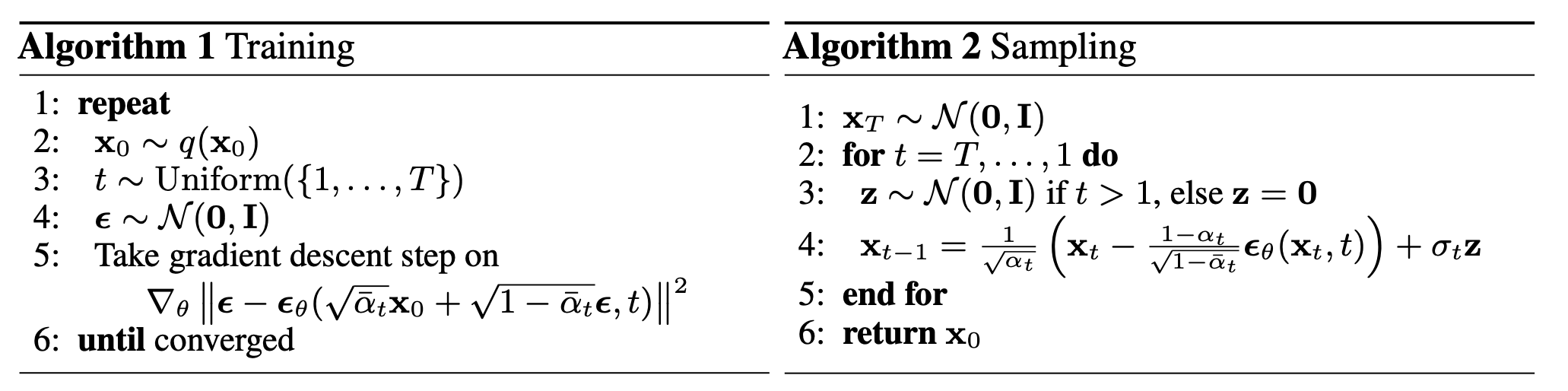
Training Algorithm

The integration over \(x_{0:T}\) can be approximated by sampling discrete samples according to the joint distribution \(q(x_{0:T} )\). Since \(q(x_{0:T} ) = \prod_{t=1}^T q(x_t \| x_{t-1}) q(x_0)\), we can firstly sample \(x_0\) from the training dataset according to \(q(x_0)\), and then sample \(x_{1:T}\) from the Markov chain. A gradient descent step is computed from the loss function upper bound above and then we re-sample \(x_{0:T}\) for the next iteration.

As we sample \(x_0\) randomly from the training dataset, we actually assume that the samples in the training set are independently and identically distributed. Otherwise, the sampling probability will be different from \(q(x_0)\). Therefore, it is important to collect data samples with good density, coverage and diversity. Otherwise, the maximium likelihood estimation loss will be biased.

Reference

Deep Unsupervised Learning using Nonequilibrium Thermodynamics

Denoising Diffusion Probabilistic Models

https://ayandas.me/blog-tut/2021/12/04/diffusion-prob-models.html