Optimization for Least Square Problems
- The Problem Definition
- Newton’s Method
- Line Search - Gauss-Newton Method
- Trust Region - The Levenberg–Marquardt Method
- The Golden Bundle Adjustment (BA)
- Generalized Least Squares
- Reference
The Problem Definition
The problem is to find solutions to a system of equations that have the form:
\[f_1(\mathbf{x}) = 0,\] \[f_2(\mathbf{x}) = 0,\] \[f_3(\mathbf{x}) = 0,\] \[...\] \[f_m(\mathbf{x}) = 0,\]where \(\mathbf{x} = [x_1, x_2, ..., x_n]^T\) is a \(n\)-dimensional vector. For convenience, we denote \((f_1, f_2, ..., f_m)^T\) by a vector-valued function \(\mathbf{f}\) and \(\mathbf{f}\) can be nonlinear functions. Then the system of equations can be re-written as
\[\mathbf{f}(\mathbf{x}) = 0,\]i.e., we wish to find a vector that makes the vector function equal to the zero vector. Since it is the general case that \(m\) is larger that \(n\), i.e., the system of equations is overdetermined, the problem would infeasible. Therefore, the alternative is to find the optimal solution which minimizes the sum of the least squares which is also the objective of the least squares problem:
\[F(\mathbf{x}) = \frac{1}{2} \sum_{i=1}^m \|f_i(\mathbf{x}) \|_2^2 = \frac{1}{2} \mathbf{f}(\mathbf{x})^T \mathbf{f}(\mathbf{x}).\]Terminalogy
The first and second derivatives of the objective function are given below:
\[\nabla F(\mathbf{x}) = F'(\mathbf{x}) = \mathbf{f}(\mathbf{x})^T \mathbf{J}(\mathbf{x}),\]where \(\mathbf{J}(\mathbf{x})\) is the \(m \times n\) jacobian matrix of the transformation \(\mathbf{f} : \mathbb{R}^m \times \mathbb{R}^n\).
\[\nabla^2 F(\mathbf{x}) = F''(\mathbf{x}) = \mathbf{J}(\mathbf{x})^T \mathbf{J}(\mathbf{x}) + \sum_{i=1}^m f_i(\mathbf{x}) \mathbf{H}_i(\mathbf{x}),\]where \(\mathbf{H}_i(\mathbf{x}) = f_i''(\mathbf{x})\) is the \(n \times n\) Hessian matrix of the scalar-valued function \(f_i(\mathbf{x})\).
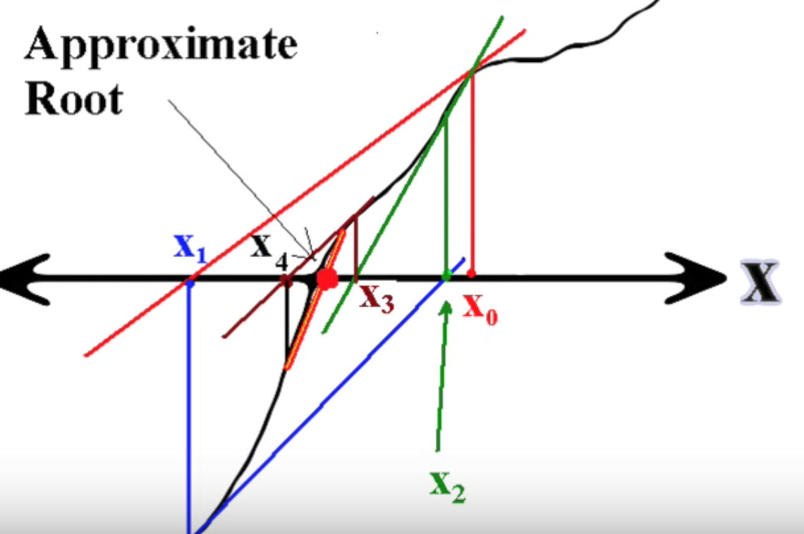
Newton’s Method
Newton’s method is an algorithm originally designated to locate roots of equations, e.g., \(F(\mathbf{x})=0\). It is derived from the linear approximation of the function \(F(\mathbf{x})\) by first-order Tayor series expansion. From Calculus, the following is the linear approximation of \(F(\mathbf{x})\) at \(\mathbf{x}+\mathbf{h}\):
\[F(\mathbf{x} + \mathbf{h}) \approx F(\mathbf{x}) + F'(\mathbf{x}) \mathbf{h},\]if \(\|\mathbf{h}\|\) is sufficiently small. By rearranging the equation, we obtain
\[F(\mathbf{x}) \approx F(\mathbf{x}_t) + F'(\mathbf{x}_t) (\mathbf{x} - \mathbf{x}_{t}) = 0.\]The update step is explicitly written as
\[\mathbf{x}_{t+1} = \mathbf{x}_{t} - \left[ F'(\mathbf{x}_{t})^T F'(\mathbf{x}_{t}) \right]^{-1} F'(\mathbf{x}_{t})^T F(\mathbf{x}_{t}) \equiv \mathbf{x}_t + \mathbf{h}.\]
Connection between Newton’s method and optimization. Newton’s method can also be used as a descent method for iterative non-linear optimization: from a starting point \(\mathbf{x}_0\) it produces a series of vectors \(..., \mathbf{x}_t, \mathbf{x}_{t+1},...\) which (hopefully) converges to \(\mathbf{x}^*\), a local stationary minimizer for the given function \(F(\mathbf{x})\). Since \(\mathbf{x}^*\) is a stationary point, it satisfies \(F'(\mathbf{x}^*) = 0\). Similarly, we have
\[F'(\mathbf{x}+\mathbf{h}) \approx F'(\mathbf{x}) + F''(\mathbf{x}) \mathbf{h},\]Here the Newton’s method is used to locate the root of \(F'(\mathbf{x}^*) = 0\). The update step is
\[\mathbf{x}_{t+1} = \mathbf{x}_t + \mathbf{h}_N,\]where \(\mathbf{h}_N\) is the solution to
\[F'(\mathbf{x}) + F''(\mathbf{x}) \mathbf{h} = 0.\]If \(F''(\mathbf{x})\) is positive definite, \(\mathbf{h}_N^T F''(\mathbf{x}) \mathbf{h}_N = - \mathbf{h}_N^T F'(\mathbf{x}) > 0\), which means \(\mathbf{h}_N\) is a descent direction when minimizing \(F(\mathbf{x})\). Therefore, Newton’s method is only useful in the final stage of the iteration where \(\mathbf{x}\) is close to \(\mathbf{x}^*\) so that \(F''(\mathbf{x})\) is positive definite. The good news about Newton’s method is that if \(F''(\mathbf{x})\) is positive definite, we get quadratic convergence while gradient descent (the steepest descent method) can only produce linear convergence.
Line Search - Gauss-Newton Method
The Gauss-Newton method is based on the linear approximation to \(\mathbf{f}\) by the first-order Tayor series expansion in the neighbourhood of \(\mathbf{x}\): For small \(\|\mathbf{h}\|\), we have
\[\mathbf{f}(\mathbf{x} + \mathbf{h}) = \ell(\mathbf{h}) \approx \mathbf{f}(\mathbf{x}) + \mathbf{J}(\mathbf{x}) \mathbf{h},\]where \(\mathbf{J}(\mathbf{x})\) is the Jacobian matrix of \(\mathbf{f}(\mathbf{x})\). Then
\[F(\mathbf{x} + \mathbf{h}) = L(\mathbf{h}) = \frac{1}{2} \ell(\mathbf{h})^T \ell(\mathbf{h})\] \[\approx \frac{1}{2} \mathbf{f}^T\mathbf{f} + \mathbf{h}^T\mathbf{J}^T\mathbf{f} + \frac{1}{2} \mathbf{h}^T \mathbf{J}^T\mathbf{J}\mathbf{h}\] \[=F(\mathbf{x}) + \mathbf{h}^T\mathbf{J}^T\mathbf{f} + \frac{1}{2} \mathbf{h}^T \mathbf{J}^T\mathbf{J}\mathbf{h},\]where \(\mathbf{f} = \mathbf{f}(\mathbf{x})\) and \(\mathbf{J} = \mathbf{J}(\mathbf{x})\).
There is a little interesting fact to address here. If we directly apply the second-order taylor expansion to \(F(\mathbf{x})\), we get
\[F(\mathbf{x} + \mathbf{h}) = L(\mathbf{h}) = F(\mathbf{x}) + \mathbf{h}^T\mathbf{J}^T\mathbf{f} + \frac{1}{2} \mathbf{h}^T \mathbf{H}\mathbf{h},\]where \(\mathbf{H}\) is the Hessian matrix at current \(\mathbf{x}\). Since the Hessian matrix is generally hard to compute, the square of jacobian \(\mathbf{J}^T\mathbf{J}\) is often used to approximate the Hessian matrix \(\mathbf{H}\). As shown by the second equation in Terminalogy, the approximation just eliminates the second term \(\sum_{i=1}^m f_i(\mathbf{x}) \mathbf{H}_i(\mathbf{x})\).
Getting back to the point, the Gauss-Newton step is to minimize \(L(\mathbf{h})\), i.e., the objective at next point,
\[\mathbf{h}_{GN} = \arg\min_{\mathbf{h}} L(\mathbf{h}).\]It is easily seen that the gradient and the Hessian of \(L\) with respect to \(\mathbf{h}\) are
\[L'(\mathbf{h}) = \mathbf{f}^T\mathbf{J} + \mathbf{h}^T \mathbf{J}^T \mathbf{J},\] \[L''(\mathbf{h}) = \mathbf{J}^T \mathbf{J}.\]We can see that \(L''(\mathbf{h})\) is independent of \(\mathbf{h}\). If \(\mathbf{J}\) is full rank, i.e., if the columns are linearly independent, then \(L''(\mathbf{h})\) is positive definite, which means \(L(\mathbf{h})\) is convex. Inspired by Newton’s method, the minimization problem can be solved by finding \(\mathbf{h}\) that makes \(L'(\mathbf{h}) = \mathbf{0}\), i.e.
\[(\mathbf{J}^T \mathbf{J}) \mathbf{h}_{GN} = - \mathbf{J}^T\mathbf{f}.\]This is a descent direction for \(F\) since
\[\mathbf{h}_{GN}^T F'(\mathbf{x}) = \mathbf{h}_{GN}^T (\mathbf{J}^T \mathbf{f}) = - \mathbf{h}_{GN}^T (\mathbf{J}^T \mathbf{J})\mathbf{h}_{GN} < 0.\]The update step of the Gauss-Newton method is typically:
\[\text{Solve}\,\,\,\, (\mathbf{J}^T \mathbf{J}) \mathbf{h}_{GN} = - \mathbf{J}^T\mathbf{f},\] \[\mathbf{x}_{t+1} = \mathbf{x}_t + \alpha \mathbf{h}_{GN},\]where \(\alpha\) is found by line search. The classical Gauss-Newton method uses \(\alpha = 1\) in all steps. In general, the Gauss-Newton method ensure linear convergence \((\|\mathbf{x}_{t+1} - \mathbf{x}^* \| \leq a\|\mathbf{x}_t - \mathbf{x}^* \|, 0 < a < 1)\) and even quadratic convergence \((\|\mathbf{x}_{t+1} - \mathbf{x}^* \| = O(\|\mathbf{x}_t - \mathbf{x}^* \|^2))\) when \(\mathbf{x}\) is close to \(\mathbf{x}^*\).
The method of locating the direction by solving \(L'(\mathbf{h}) = 0\) is called exact line search. An alternative is inexact line search which loosely asks for a sufficient decrease in \(L(\mathbf{h})\), e.g., using backtracking line search or Wolfe conditions to loosely find step length along given search direction.
Trust Region - The Levenberg–Marquardt Method
The LM method suggests to use a damped Gauss-Newton mothod. The step \(\mathbf{h}_{LM}\) is defined by the following modification:
\[(\mathbf{J}^T \mathbf{J} + \mu \mathbf{I}) \mathbf{h}_{LM} = - \mathbf{J}^T\mathbf{f} \text{ and } \mu \geq 0.\]The damping parameter \(\mu\) has several effects:
- For all \(\mu > 0\) the coefficient matrix \(\mathbf{J}^T \mathbf{J} + \mu \mathbf{I}\) is positive definite, and this ensures that \(\mathbf{h}_{LM}\) is a descent direction.
- For large values of \(\mu\) we get \(\mathbf{h}_{LM} = -\frac{1}{\mu} \mathbf{J}^T\mathbf{f} = -\frac{1}{\mu} F'(\mathbf{x}),\) i.e. a short step in the steepest descent direction. This is desired if the current iterate is far from the solution. But, the larger damping factor \(\mu\) is, the slower convergence gets.
- For small values of \(\mu\), \(\mathbf{h}_{LM} = \mathbf{h}_{GN}\), which is a good step in the final stage of the iteration. When \(\mathbf{x}\) is close to \(\mathbf{x}^*\), the LM can have almost quatratic final convergence as the Gauss-Newton method.
Thus, the damping parameter influences both the direction and the size of the update step. This leads us to make a method without a specific line search (i.e., to explicitlt determine the step size).
The Golden Bundle Adjustment (BA)
Bundle Adjustment (BA) is a classic optimization problem developed in photogrammetry in the 50’s. Each error function corresponds to a reprojection error concerning a camera and a 3D point.
Suppose a BA problem considers a set of \(m\) cameras \(\mathcal{C} = \{c_1, c_2, \ldots, c_m \}\), a set of \(n\) points \(\mathcal{P}= \{p_1, p_2, \ldots, p_n \}\) and a set of projections \(\mathcal{E} \in \mathcal{C} \times \mathcal{P}\), the objective is to estimate the \((m+n)\)-dimensional vector \(\mathbf{x} = [c_1, c_2, \ldots, c_m, p_1, p_2, \ldots, p_n]^T\). The total \(k\) reprojection functions form a \(k\) dimensional vector denoted by \(\mathbf{e} = [e_1, e_2, \ldots, e_k]^T\). The Jacobian matrix is computed by taking the first-order derivative of the error vector \(\mathbf{e}\) with respect to the input vector \(\mathbf{x}\):
\[\mathbf{J}_{k \times (m+n)} = \Big[ \frac{\partial \mathbf{e} }{\partial c_1}, \ldots, \frac{\partial \mathbf{e} }{\partial c_m}, \frac{\partial \mathbf{e} }{\partial p_1}, \ldots, \frac{\partial \mathbf{e} }{\partial p_n} \Big] \equiv \Big[ \mathbf{J}_{c_1}, \ldots, \mathbf{J}_{c_m}, \mathbf{J}_{p_1}, \ldots, \mathbf{J}_{p_n} \Big] \equiv \Big[ \mathbf{J}_{c}, \mathbf{J}_{p} \Big].\]Based on the LM algorithm elaborated above, the update step is to solve the equation:
\[(\mathbf{J}^T \mathbf{J} + \mu \mathbf{I} ) \Delta \mathbf{x} = - \mathbf{J}^T\mathbf{e}.\]The symmetric matrix \(\mathbf{J}^T \mathbf{J}\) is quite sparse because each reprojection error function only involves one camera and one track. Here it can be re-written as
\[\mathbf{J}^T \mathbf{J} = \left[ {\begin{array}{cc} \mathbf{J}_c^T \mathbf{J}_c & \mathbf{J}_c^T \mathbf{J}_p \\ \mathbf{J}_p^T \mathbf{J}_c & \mathbf{J}_p^T \mathbf{J}_p \\ \end{array} } \right].\]For simplicity, the damping term \(\mu \mathbf{I}\) is omitted here, so that the update equation is turned into
\[\left[ {\begin{array}{cc} \mathbf{J}_c^T \mathbf{J}_c & \mathbf{J}_c^T \mathbf{J}_p \\ \mathbf{J}_p^T \mathbf{J}_c & \mathbf{J}_p^T \mathbf{J}_p \\ \end{array} } \right] \left[ {\begin{array}{cc} \Delta \mathbf{c} \\ \Delta \mathbf{p} \\ \end{array} } \right] = \left[ {\begin{array}{cc} -\mathbf{J}_c^T \mathbf{e} \\ -\mathbf{J}_p^T \mathbf{e} \\ \end{array} } \right].\]Schur Complement trick
Now, the problem is to solve the linear equation system of this form:
\[\left[ {\begin{array}{cc} B & E \\ E^T & C \\ \end{array} } \right] \left[ {\begin{array}{cc} \Delta y \\ \Delta z \\ \end{array} } \right] = \left[ {\begin{array}{cc} u \\ w \\ \end{array} } \right].\]Its solution is obtained as the solution of
\[\left[ B-EC^{-1}E^T \right] \Delta y = u - E C^{-1} w,\] \[\Delta z = C^{-1}(w - E^T \Delta y)\]by using the Schur Complement. And the first equation can then be solved by applying Cholesky factorization ( \(\mathbf{A} \mathbf{x} = \mathbf{b}\) \(\Rightarrow\) \(\mathbf{L} \mathbf{L}^T \mathbf{x} = \mathbf{b}\) \(\Rightarrow\) Solve \(\mathbf{y}\) in \(\mathbf{L} \mathbf{y} = \mathbf{b}\) \(\Rightarrow\) Solve \(\mathbf{x}\) in \(\mathbf{L}^T \mathbf{x} = \mathbf{y}\) ). Depending on the sparsity of the matrix, Cholesky factorization can be implemented in dense, sparse and iterative ways.
Conditioning of BA
The BA problem is generally known to be ill-conditioned, because of the varying sensativity of the objective function to different parameters. For example, small changes in the translation of a camera affect the objective much less than small changes in the radial distortion parameters. (See Visibility Based Preconditioning for Bundle Adjustment)
Parameters (e.g. of ceres solver)
| name | option | description |
|---|---|---|
| minimizer type | TRUST_REGION | first direction, second step size |
| LINE_SEARCH | first step size, second direction | |
| line search direction type | LBFGS | LINE_SEARCH requires the computation of Hessian. LBFGS approximates the inverse of Hessian by a low-rank positive-definite matrix. |
| line search type | WOLFE | solve inexact line search using Wolfe conditions |
| nonlinear conjugate gradient type | FLETCHER_REEVES | Fletcher–Reeves evaluates the increments of each iteration: \(\Delta \mathbf{x}\) |
| max lbfgs rank | 20 | Limited-memory BFGS constrains the rank of approximate inverse Hessian to be below 20 for memory efficiency. |
| use approximate eigenvalue bfgs scaling | false | BFGS initially takes the inverse Hessian approximation to be identity. It rescales the approximation by a eigenvalue of the true inverse Hessian. |
| line search interpolation type | CUBIC/BISECTION/QUATRATIC | Interpolation methods are a kind of line search methods. It fits the loss \(f(x+\alpha\Delta x)\) by quatratic or cubic polynomial in \(\alpha\). It leads to easier computation of derivatives and so on. |
| min line search step size | 1e-9 | |
| line search sufficient function decrease | 1e-4 | |
| max line search contraction | 1e-3 | The update is written as \(s_t = \alpha \Delta x + \beta s_{t-1}\). The contraction \(\beta\) is a multiplier of last step. 0 < max_step_contraction < min_step_contraction < 1. |
| min line search contraction | 0.6 | |
| max num line search step size iterations | 20 | Max number of trials of finding a satisfying step size in each iteration. |
| max num line search direction restarts | 5 | Maximum number of restarts of the line search direction |
| line search sufficient curvature_decrease | 0.9 | Wolfe conditions require a step size to satisfy |f’(step_size)| <= sufficient_curvature_decrease * |f’(0)|. |
| max line search step expansion | 10.0 | Wolfe conditions require new_step_size <= max_step_expansion * step_size. |
| trust region strategy type | LEVENBERG_MARQUARDT | |
| Dogleg Type | TRADITIONAL_DOGLEG | LM works with combinations of Gauss-Newton and steepest descent directions. Dogleg methods find an approximate step of LM by combining the steps of both. |
| use nonmonotonic steps | false | Allow the objective to increase so that the optimization can “jump over boulders” rather than moving into narrow valleys. |
| max consecutive nonmonotonic steps | 5 | |
| min lm diagonal | 1e-6 | For LM, the scaled diagonal of \(J^TJ\) is used to control the size of trust region. The diagonal values need to be clamped to ensure successful regularization. |
| max lm diagonal | 1e32 | |
| linear solver type | SPARSE NORMAL CHOLESKY | |
| DENSE QR | ||
| preconditioner type | JACOBI | 关于预调节器(preconditioner)的理解,请参考知乎帖子 |
| CLUSTER_JACOBI | ||
| CLUSTER_TRADITIONAL | ||
| linear solver ordering | In bundle adjustment, points are desired to have an order prior to cameras. | |
| use postordering | false | Sparse Cholesky factorization permutes the columns and then computes the jacobian or do the inverse. |
| use inner iterations | false | Once the Newton/Trust Resion step has been computed for all params, the inner iterations will further optimize them from this starting point. |
| inner iteration ordering | Specify the order of variable steps to be optimized. | |
| jacobi scaling | true | Normalize the jacobian using Jacobi scaling before calling the linear least squares solver. |
Generalized Least Squares
Here, we consider a regression problem: Given a set of observation data \(\{(\mathbf{x}_i, \mathbf{y}_i)\}_{i=1,..,n}\), we want to regress a linear/nonlinear function \(\mathbf{f}(.)\) which minimizes
\[\sum_{i=1}^n |\mathbf{y}_i - \mathbf{f}(\mathbf{x}_i)|_2^2.\]The assumption is generally held that the condifition mean of \(\mathbf{Y}\) given \(\mathbf{X}\) is equal to \mathbf{f}(\mathbf{X}) and the conditional variance-covariance of \(\mathbf{Y}\) given \(\mathbf{X}\) is a known nonsingular matrix \(\mathbf{\Omega}\). Therefore, the conditional mean and covariance of the error term \(\mathbf{\epsilon} = \mathbf{Y} - \mathbf{f}(\mathbf{X})\) are zero and \(\mathbf{\Omega}\), i.e.,
\[E(\mathbf{\epsilon} | \mathbf{X}) = 0, C(\mathbf{\epsilon} | \mathbf{X}) = \mathbf{\Omega}.\]Therefore, the generalized least square problem is formulated as
\[\min (\mathbf{Y} - \mathbf{f}(\mathbf{X}))^T \Omega^{-1} (\mathbf{Y} - \mathbf{f}(\mathbf{X})),\]which minimizes the squared Mahalanobis length of this residual vector \(\mathbf{\epsilon}\).
Since the covariance \(\mathbf{\Omega}\) is generally unvailable, the Feasible Generalized Least Squares (FGLS) estimator is adopted. It proceeds in two stages:
-
the model is estimated by Ordinary Least Squares (OLS) and the residuals are used to build a consistent estimator of the errors covariance matrix \(\mathbf{\Omega}\);
-
using the estimated \(\mathbf{\Omega}\), solve the generalized least square problem.
Covariance Estimation [3][4]
“One way to assess the quality of the solution returned by a non-linear least squares solver is to analyze the covariance of the solution.” Let’s consider
\[\mathbf{f}(\mathbf{x}) = \mathbf{\epsilon} \sim N(0, \mathbf{S}).\]Taking the first-order taylor expansion of \(\mathbf{f}(\mathbf{x})\), we have
\[\mathbf{f}(\mathbf{x}_t) + \mathbf{J} (\mathbf{x} - \mathbf{x}_t) = \mathbf{\epsilon}.\]Therefore, the covariance of \(\mathbf{\epsilon}\), \(C(\mathbf{\epsilon}) = \mathbf{J} C(\mathbf{x}) \mathbf{J}^T\). Then we get \(C(\mathbf{x}) = \mathbf{J}^{-1} C(\mathbf{\epsilon}) \mathbf{J}^{-T} = \mathbf{J}^{-1} \mathbf{S} \mathbf{J}^{-T}\). If we assume the error vector takes identity covariance (iid), i.e., \(\mathbf{S} = \sigma^2 \mathbf{I}\), the covariance of the variable \(\mathbf{x}\) becomes \(C(\mathbf{x}) = \sigma^2 \mathbf{J}^{-1} \mathbf{J}^{-T} = \sigma^2 (\mathbf{J}^T \mathbf{J})^{-1}\).
Reference
[1] Nonlinear Systems - Newton’s Method
[2] METHODS FOR NON-LINEAR LEAST SQUARES PROBLEMS
[3] Covariance estimation reference 1
[4] Covariance estimation reference 2
[5] HESSIAN MATRIX VS. GAUSS–NEWTON HESSIAN MATRIX
[6] Pushing the Envelope of Modern Methods for Bundle Adjustment
[7] Bundle Adjustment in the Large
[8] Generalized Subgraph Preconditioners for Large-Scale Bundle Adjustment
[9] Tutorial on computing Jacobian for Bundle Adjustment Problem - Part1
[9] Tutorial on computing Jacobian for Bundle Adjustment Problem - Part2
[10] Indicative parameter setting for LM based Bundle Adjustment
[11] METHODS FOR NON-LINEAR LEAST SQUARES PROBLEMS
[12] A review of trust region algorithms for optimization
[13] Pushing the Envelope of Modern Methods for Bundle Adjustment
[14] Bundle Adjustment in the Large
[15] Visibility Based Preconditioning for Bundle Adjustment
[16] Distributed Very Large Scale Bundle Adjustment by Global Camera Consensus
[17] A Consensus-Based Framework for Distributed Bundle Adjustment
[18] pOSE: Pseudo Object Space Error for Initialization-Free Bundle Adjustment
[19] ICE-BA: Incremental, Consistent and Efficient Bundle Adjustment for Visual-Inertial SLAM
[20] Is Levenberg-Marquardt the Most Efficient Optimization Algorithm for Implementing Bundle Adjustment?
[22] Sparse sparse bundle adjustment
[23] Multicore Bundle Adjustment