CNN Networks
Milestone CNN Networks
| CNN Networks | Year | First Author | Max Depth | Max Params | Originality |
|---|---|---|---|---|---|
| Lenet | 1998 | Yann LeCun | 7 | 11880+ | |
| AlexNet | 2012 | Alex Krizhevsky | 8 | 60M | Dropout |
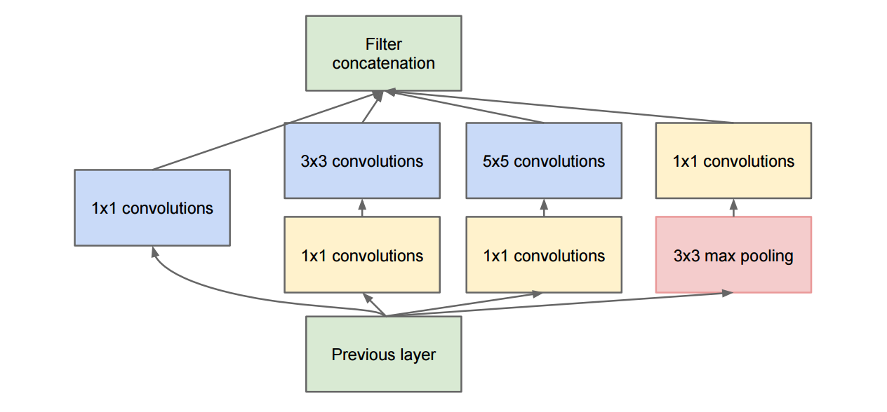
| GoogLenet | 2014 | Christian Szegedy | 22 | Inception module (Fig. 1); Intermediate classifier | |
| VGG | 2014 | Karen Simonyan | 19 | 144M | 3\(\times\)3 kernels |
| ResNet | 2015 | Kaiming He | 152 | Residual learning; Shortcuts |
Other Networks
| CNN Networks | Year | First Author | Originality |
|---|---|---|---|
| NIN | 2013 | Min Lin | Mlpconv (Fig. 2) & Global average pooling |
| Maxout Network | 2013 | Ian J. Goodfellow | Max pooling over affine feature maps |
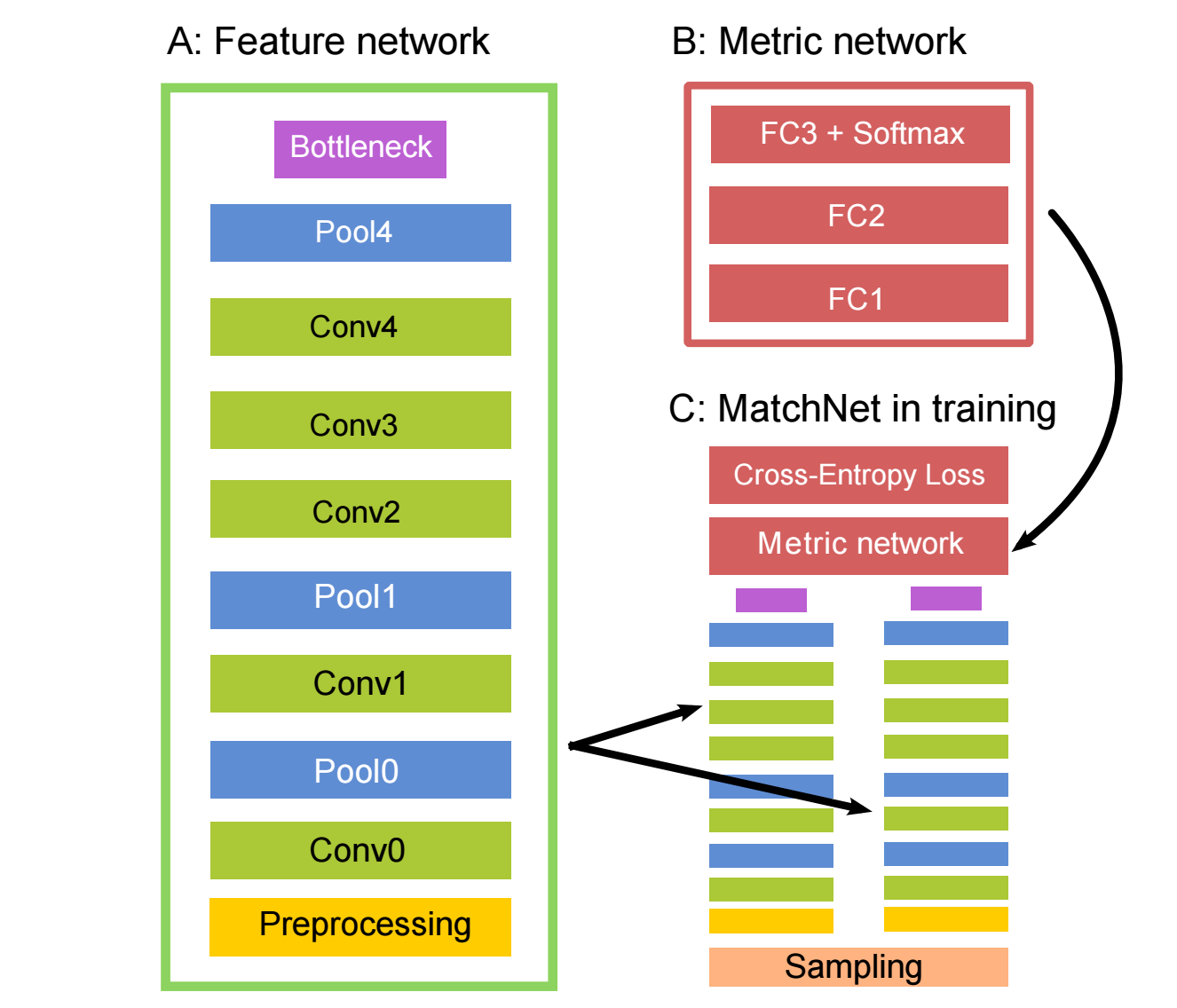
| MatchNet | 2015 | Xufeng Han | Produce similarity score for patch pair (Fig. 3) |
| Spatial Transformer Network | 2015 | Max Jaderberg | Spatial transformer module (Fig. 4) |
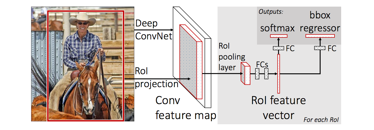
| Fast R-CNN | 2015 | Ross Girshick | Share computation compared to R-CNN (Fig. 5) |
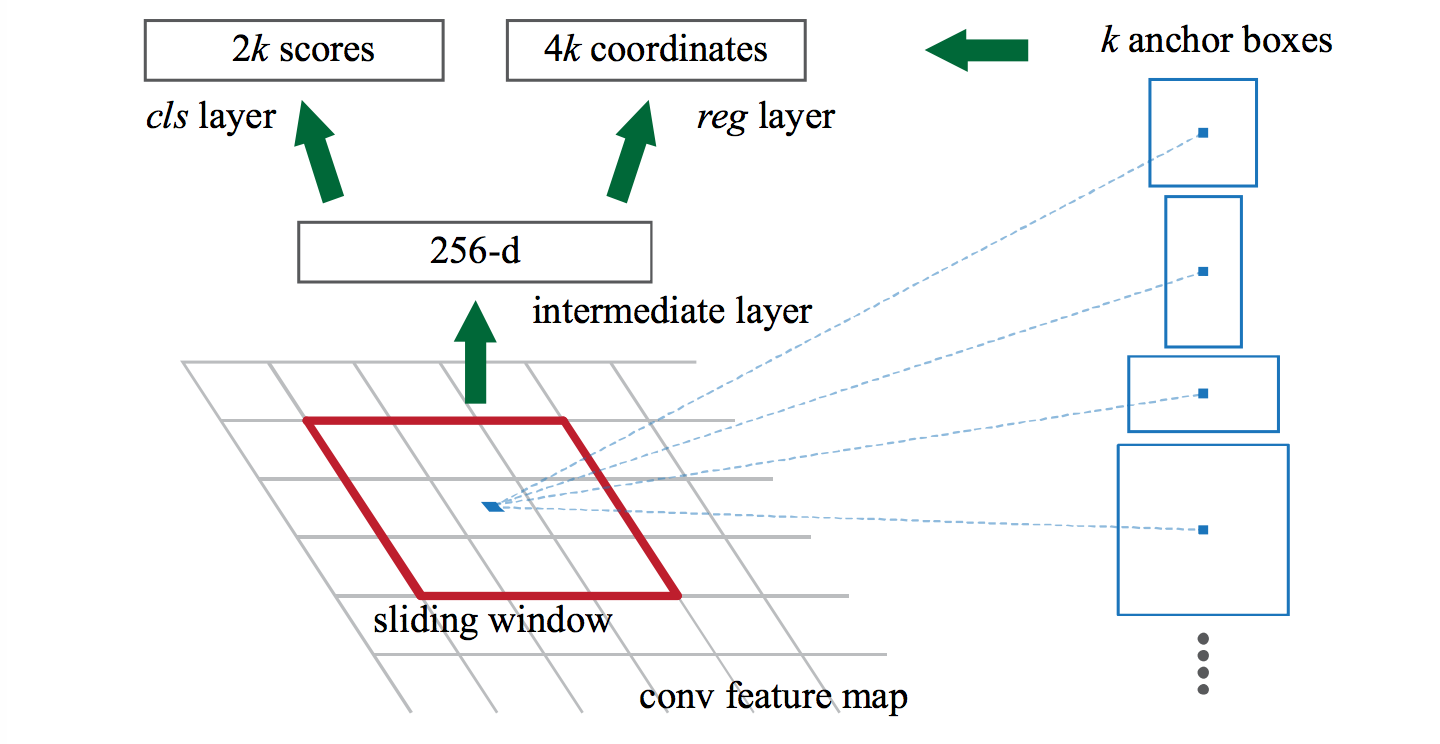
| RPN | 2015 | Shaoqing Ren | Region Proposal Network (Fig. 6) |
Deep Inside CNN
- Deep Inside Convolutional Networks: Visualising Image Classification Models and Saliency Maps (to read)
- Visualizing and Understanding Convolutional Networks (to read)
Reflections
-
Fully convolutional network is equivalent to InnerProduct matrix multiplication layer, since each element of the output vector equals the weighted sum of all input feature map pixels.
- 卷积层的weights要共用,feature map的数量一定要一致,但是spatial size没有要求。
- In NIN, it says that the convolution filters in CNN is generalized linear model (GLM) for the underlying data patch and the level of abstraction is low with GLM. By abstraction, in means that the feature is invariant to the variants to the same concept. Therefore, high invariance necessitates abstraction, i.e., nonlinearity mathematically of CNN functions. In conventional CNN, the deficient nonlinearity of convolution filters is compensated by utilizing an over-complete set of filters to cover all variations of the latent concepts.
Appendix
| Layer | Shape | Output Blob Shape |
|---|---|---|
| input | 3x227x227 | |
| conv1 | 96x11x11,stride=4 | 1x96x55x55 |
| pool1 | 3x3,stride=2 | 1x95x27x27 |
| conv2 | 256x5x5,stride=1 | 1x256x27x27 |
| pool2 | 3x3,stride=2 | 1x256x13x13 |
| conv3 | 384x3x3,stride=1 | 1x384x13x13 |
| conv4 | 384x3x3,stride=1 | 1x384x13x13 |
| conv5 | 256x3x3,stride=1 | 1x256x13x13 |
| pool5 | 3x3,stride=2 | 1x256x6x6 |
| fc6 | 4096 | |
| fc7 | 4096 | |
| fc8 | 1000 |
| Layer | Shape | Output Blob Shape |
|---|---|---|
| input | 1x64x64 | |
| conv1 | 24x7x7,stride=1 | 1x24x64x64 |
| pool1 | 3x3,stride=2 | 1x24x32x32 |
| conv2 | 64x5x5,stride=1 | 1x64x32x32 |
| pool2 | 3x3,stride=2 | 1x64x16x16 |
| conv3 | 96x3x3,stride=1 | 1x96x16x16 |
| conv4 | 96x3x3,stride=1 | 1x96x16x16 |
| conv5 | 64x3x3,stride=1 | 1x64x16x16 |
| pool5 | 3x3,stride=2 | 1x64x8x8 |
| Layer | Shape | Output Blob Shape |
|---|---|---|
| input | 3x224x224 | |
| conv1_1 | 64x3x3,stride=1 | 1x64x224x224 |
| conv1_2 | 64x3x3,stride=1 | 1x64x224x224 |
| pool1 | 2x2,stride=2 | 1x64x112x112 |
| conv2_1 | 128x3x3,stride=1 | 1x128x112x112 |
| conv2_2 | 128x3x3,stride=1 | 1x128x112x112 |
| pool2 | 2x2,stride=2 | 1x128x56x56 |
| conv3_1 | 256x3x3,stride=1 | 1x256x56x56 |
| conv3_2 | 256x3x3,stride=1 | 1x256x56x56 |
| conv3_3 | 256x3x3,stride=1 | 1x256x56x56 |
| pool3 | 2x2,stride=2 | 1x256x28x28 |
| conv4_1 | 512x3x3,stride=1 | 1x512x28x28 |
| conv4_2 | 512x3x3,stride=1 | 1x512x28x28 |
| conv4_3 | 512x3x3,stride=1 | 1x512x28x28 |
| pool4 | 2x2,stride=2 | 1x512x14x14 |
| conv5_1 | 512x3x3,stride=1 | 1x512x14x14 |
| conv5_2 | 512x3x3,stride=1 | 1x512x14x14 |
| conv5_3 | 512x3x3,stride=1 | 1x512x14x14 |
| pool5 | 2x2,stride=2 | 1x512x7x7 |
| fc6 | 4096 | |
| fc7 | 4096 | |
| fc8 | 1000 |


 Figure5. Fast R-CNN architecture The inputs are a whole image and a set of object proposals. It first processes image to produce a conv feature map and then extracts a fixed-length vector from the feature map for each proposal.Two subsequent sibling branches produce classification probability and refined bounding box respectively for proposals.
 Figure6. Region Proposal Network The sliding n\(\times\)n window is mapped to a lower-dimensional vector by an n\(\times\)n conv layers, followed by two sibling 1\(\times\)1 conv layers and fully-connected layers for box regression and box classification respectively.