Belief Propagation

Introduction

A short definition of belief propagation in one sentence is that it is a message passing algorithm for performing inference on graphical models. The inference process aims to estimate the marginals of variable nodes of the probability graph, i.e., to figure out the probabilistical distribution of nodes’ underlying states or labels.

To make life easy, I start my exposition by re-stating a pretty simple example I have learned from Quora [2]. First, let’s look at the factor graph as shown below.

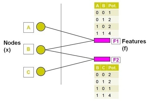
It is a bipartite graph comprising two types of nodes: the variable nodes (A, B, C on the left side) and the factor nodes (F1, F2 on the right side). The structure of the fractor graph illustrates the fractorization of origin probability graph into (A, B) and (B, C). The factor nodes fractorize the graph into small pieces and each of them maintains a table of the local joint probabilities of associated variable nodes. The task here is to estimate the marginal probabilities of A, B and C which assumes binary states using BP. The naive algorithm is to calculate the joint probability of the variables that encompasses \(2^3\) possibilities as shown below.

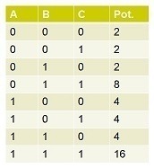
The last column denotes the potential of each possibility. By summing out the cases, it would be direct to compute that \(P(A=0)=14/42=1/3\), \(P(B=0)=12/42=2/7\) and \(P(C=0)=12/42=2/7\). Since it is intractable to compute the joint probability when the number of variables gets large, the BP considers the message passing inside factor graph. In BP, each variable node sends a message to its neighboring factor node and vice versa. The message is basically the belief about some variable node’s probability of being 0 or 1. It is recorded by two potential values without normalization like \((14, 28)\) or \((12, 30)\). The main step of BP is about passing messages between variable nodes and factor nodes iteratively: a variable node \(v\) sends message to a factor node \(f\) by multiplying all the messages it gets from its neighboring factor nodes except \(f\). Intuitively, it tells \(f\) what other factor nodes think about its probability of being 0 or 1. A factor node \(f\) sends a message to a node \(n\) by multiplying all the messages it gets from its neighboring variable node except \(n\), and then multiplying the resultant product with its own potential table. Intuitively, the message sent to \(n\) is determined by the related varible nodes sharing the same factor. It absorbs the property (like Markov property) about how the states of related variable nodes interact with each other. The detailed steps are as follows:

1. Variable node \(\rightarrow\) factor node. As the start, all variable nodes haven’t received any message from fractors, thus, they send message [1, 1] to all factors indicating the same possibility of being any states.

2. Factor node \(\rightarrow\) variable node. Considering the message passing from F1 to A, since there is only one other message from B, we don’t need to multiply anything. Then multiplying the message from B (1, 1) with F1’s potential table, we get [1, 2, 2, 4] which corresponds to [P(A=0, B=0), P(A=0, B=1), P(A=1, B=0), P(A=1, B=1)]. After summing out, F1 passes the message [P(A=0), P(A=1)] = [3, 6] = [1, 2] to A. Similarly, F1 to B is also [1, 2], F2 to B is [4, 5] and F2 to C is [1, 2].

3. Variable node \(\rightarrow\) factor node. Since A and C both have only one factor nodes connecting to them, they will always pass the initial message [1, 1] to their connected factor node F1 and F2. Node B is a little bit more complicated. Message from B to F1 is multiplication of all messages to B except from F1, i.e., the message from F2 to B, [4, 5]. Similarly, message from B to F2 is the message from F1 to B, [1, 2].

4. Factor node \(\rightarrow\) variable node. To calculate message from F1 to A, we first multiply F1’s potential table with message from B to F1 which leads to [14, 28] = [1, 2]. Similarly, F1 to B is [1, 2], F2 to B is [4, 5] and F2 to C is [2, 5].

5. Variable node \(\rightarrow\) factor node. Again, B to F1 is [4, 5], B to F2 is [1, 2].

6. As we can see, the message from variable nodes to factor nodes in iteration 5 and 3 are the same. The iterative process stops. Now we can compute the marginals of each node. By multiplying all messages sent by factor nodes, message for each node is obtained: A is [1, 2], B is [4, 10] and C is [2, 5]. Therefore, \(P(A=0)=1/3\), \(P(B=0)=2/7\), \(P(C=0)=2/7\).

Properties of BP

BP provides exact solution when there are no loops in graph (e.g. chain, tree). It can be solved by Viterbi algorithm (a dynamic programming approach). Otherwise, approaximate (but often good) solution is anticipated for loopy BP.

A graphical model with higher-order potential functions may always be converted to a graphical model with only pairwise potential functions through a process of variable augmentation, though this may also increase the nodes’ state dimension undesirably.

Convergence of BP

Application: Stereo Matching Using Belief Propagation [3]

Classical dense two-frame stereo matching computes a dense disparity or depth map from a pair of images under known camera configuration. The Bayesian stereo matching is well studied and formulated as a maximum a posteriori MRF (MAP-MRF) problem, because of the homogeneous property of local disparities. As stated in [3], the proposed solution models stereo vision by three coupled MRF’s: \(\mathbf{D}\) for smooth disparity field involving each pixel, \(\mathbf{L}\) for spatial line process involving each pair of neighboring pixels to indicate smooth discontinuity and \(\mathbf{O}\) for binary process involving each pixel to indicate occulusion. Theoretically, all the three variables \(\mathbf{D}\), \(\mathbf{L}\) and \(\mathbf{O}\) hold Markov property in image. Then the posterior is computed by

Here, in [3], two independence assumptions are adopted. First, the observations from image \(\mathbf{I}\) is independent of \(\mathbf{L}\), i.e., \(P(\mathbf{I} \| \mathbf{D}, \mathbf{L}, \mathbf{O}) = P(\mathbf{I} \| \mathbf{D}, \mathbf{O})\). Second, statistical dependence between \(\mathbf{O}\) and \(\{\mathbf{D}, \mathbf{L}\}\) is ignored, i.e., \(P(\mathbf{D}, \mathbf{L}, \mathbf{O}) = P(\mathbf{D}, \mathbf{L})P(\mathbf{O})\).

For the likelihood part, only the matching cost of each pixel \(s\) with disparity \(d_s\) in non-occulusion region is condidered. It results in

For the prior part, the line process penalizes difference in disparities between neighboring pixels if discontinuity does not occur and penalize the occurrence of discontinuity otherwise:

and

The prior of occulusion is simply modeled as \(P(\mathbf{O}) = \prod_s exp(-\eta_c(o_s))\) to penalize the occurrence of occulusion.

To sum up, the MAP problem can be written as

By properly defining robust functions, the occulusion constraint and continuity constraint can be converted into implicit constraints and the problem will be changed into

After the formulation, loopy belief propagation is applied to solve the problem approximately.

Reference

[1] A Tutorial Introduction to Belief Propagation

[2] Quara answer

[3] Stereo Matching Using Belief Propagation