Discriminative Modeling VS Generative Modeling
Introduction
Generally speaking, there are two main modeling approaches in machine learning: discriminative modeling (DM, e.g., the naive Bayes and HMM) and generative modeling (GM, e.g., the logistic regression model). Given two vatiables \(X \in \mathcal{X}\) (usually the observations or feature vectors) and \(Y \in \mathcal{Y}\) (usually the latent variables or labels), DM focuses on the relationship between the \(x\) and \(y\), more concretely, \(p(Y \| X)\). In other words, DM describes how to take a feature vector \(x\) and assign it to a label \(y\). GM refers to the joint distribution \(p(X, Y) = p(X \| Y) p(Y)\). It describes how a label vector \(y\) can probabilistically “generate” a feature vector \(x\).
Let us get to an inference problem where given observations \(x = (x_1, x_2, \ldots, x_K) \in \mathcal{X}\) the objective is to infer the labels \(y \in \mathcal{Y}\) from the observations.
Naive Bayes (Generative)
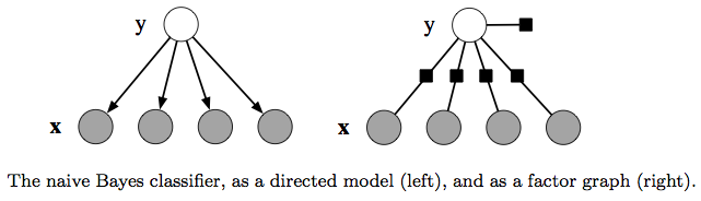
One simple way to accomplish the inference is to assume that once the class label \(y\) is known, all the features are independent. (That’s why it is called naive.) It is based on a joint probability model of the form:
\[p(\mathbf{y}, \mathbf{x}) = p(\mathbf{y}) \prod_{k=1}^K p(x_k \| \mathbf{y}).\]We use the exemplar of spam email detection to exemplify this. \(x \in \mathcal{X}\) represents the contents (the logical set of words) of a piece of email and the hidden variable \(y \in \mathcal{Y}\) is a binary value denoting whether the email is spam. The detection of spam is mathetically equivalent to calculating the \(p(Y=y \| X=x)\).
The Naive Bayes takes a roundabout way by modeling the \(p(Y)\) and \(p(X \| Y)\) and then computes
\[p(Y=1 \| X=x) = \frac{p(X=x \| Y=1)p(Y=1)} {p(X=x)},\] \[p(Y=0 \| X=x) = \frac{p(X=x \| Y=0)p(Y=0)} {p(X=x)}.\]By eliminating the common scalar \(\frac{1}{p(X=x)}\), the predicition is given by comparing the joint probability \({p(X=x, Y=1)}\) and \({p(X=x, Y=0)}\).
Logistic Regression (Discriminative)
Another well-known classifier is Logistic Regression that directly models the conditional probability directly, i.e. the \(p(Y=1 \| X)\) and \(p(Y=0 \| X)\) for the email spam example, then give the prediction from \(p(Y \| X=x)\).
The general assumaption held by logistic regresion is that the log probability, \(logp(y \| X)\), of each class is a linear function of \(X\), plus a normalization constant. This leads to the conditional distribution:
\[p(y \| X) = \frac{1}{Z(X)} exp \Big\{ \theta_y + \sum_{j=1}{K} \theta_{y, j} x_j \Big\},\]where \(Z(X)\) is a normalizing constant to yield a proper conditional distribution. By some notational tricks, the above equation can be re-written as
\[p(y \| X) = \frac{1}{Z(X)} exp \Big\{ \sum_{j=1}{K} \theta_k f_k(y, X) \Big\},\]where \(\theta = \{ \theta_k \} \in \mathbb{R}^K\) is a parameter vector and \(f_k(.,.)\) are feature functions.
HMM (Generative)
Also, an example is first introduced for interpretable elaboration of HMM. Named-entity recognition (NER) is an application of nature language preprocessing. NER is, given a sentence, to segment which words are part of an entity and to classify each entity by type like locations, people, organization, etc. The independece assumption as in Naive Bayes is improper as the named-entity labels of neighboring words are dependent.
The HMM relaxes the independence assumption to arrange the output variables in a linear chain. It models a sequence of observations \(X = \{x_t \} (t=1, \ldots, T) \in \mathcal{X}\) by assuming that there is an underlying sequence of their states \(Y = \{y_t \} (t=1, \ldots, T) \in \mathcal{Y}\). To model the joint distribution \(p(\mathbf{y}, \mathbf{x})\) tractably, an HMM makes two independence assumptions:
- Each state only depends on its immediate predecessor, i.e., each state \(y_t\) is independent of all its ancestors \(y_1, y_2, \ldots, y_{t-2}\) given the preceding state \(y_{t-1}\).
- Each observation variable \(x_t\) only depends on the current state \(y_t\).
In this way,
\[p(\mathbf{y}, \mathbf{x}) = \prod_{t=1}^T p(y_t \| y_{t-1}) p(x_t \| y_t),\]where \(p(y_1 \| y_0) = p(y_1)\).
HMMs have been used for many sequence labeling tasks in natural language processing such as part-of-speech tagging, named-entity recognition, and information extraction.
Linear-chain CRF (Discriminative)
The formal definition of Linear-chain CRF is as follows:
Let \(Y\), \(X\) be random vectors, \(\theta = \{\theta_k \} \in \mathbb{R}^K\) be a parameter vector, and \(\mathcal{F} = \{ f_k(y, y', \mathbf{x}_t) \}_{k=1}^K\) be a set of real valued feature functions. Then the linear-chain CRF is a distribution \(p(\mathbf{y} \| \mathbf{x})\) that takes the form:
\[p(\mathbf{y} \| \mathbf{x}) = \frac{1}{Z(\mathbf{x})} \prod_{t=1}^T exp\Big\{ \sum_{k=1}^K \theta_k f_k (y_t, y_{t-1}, \mathbf{x}_t) \Big\}.\]Notice that a linear chain CRF can be described as a factor graph over \(\mathbf{x}\) and \(\mathbf{y}\), i.e.,
\[p(\mathbf{y} \| \mathbf{x}) = \frac{1}{Z(\mathbf{x})} \prod_{t=1}^T \Phi_t (y_t, y_{t-1}, \mathbf{x}_t),\]where local function \(\Phi_t()\) is like potential function in MRF.
General CRF
Condifitional random field (CRF) is defined based on a factor graph \(G\) over \(X\) and \(Y\). \((X, Y)\) is a conditional random field if for any value \(X = \mathbf{x}\), the distribution \(p(\mathbf{y} \| \mathbf{x})\) factorizes according to \(G\).
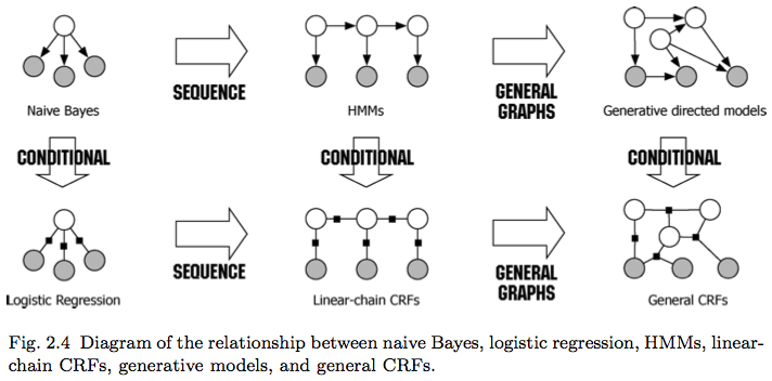
Relationships
Naive bayes and logistic regression are a generative-discriminative pair, so are HMM and linear-chain CRF. If the graph modeling the relationship of variables is directed, it’s more like generative because it models how the variables are generated. Otherwise, the undirected relationship better suites the discriminative model by getting blind to the generative process.