Image Localization
Related works
ICCV2019
-
Fine-Grained Segmentation Networks: Self-Supervised Segmentation for Improved Long-Term Visual Localization segmentation to handler season changes
-
Cascaded Parallel Filtering for Memory-Efficient Image-Based Localization filtering for matching against SfM
-
Stochastic Attraction-Repulsion Embedding for Large Scale Image Localization image retrieval
-
Is This The Right Place? Geometric-Semantic Pose Verification for Indoor Visual Localization pose verification (e.g. used in ransac), needs semantic info
-
Local Supports Global: Deep Camera Relocalization with Sequence Enhancement
-
Prior Guided Dropout for Robust Visual Localization in Dynamic Environments
Works before ICCV2019
- Neural-Guided RANSAC: Learning Where to Sample Model Hypotheses
- Feature-Based
- Tutorial
- Scene coordinate regression
- Scene Coordinate Regression Forests for Camera Relocalization in RGB-D Images
- Backtracking regression forests for accurate camera relocalization
- Random forests versus Neural Networks—What’s best for camera localization?
- DSAC DSAC-Differentiable RANSAC for camera localization
- DSAC++ Learning Less is More – 6D Camera Localization via 3D Surface Regression
- DSAC++ angle loss Scene Coordinate Regression with Angle-Based Reprojection Loss for Camera Relocalization
- Dense regression: Full-Frame Scene Coordinate Regression for Image-Based Localization: The same idea as mine
- Scene Coordinate and Correspondence Learning for Image-Based Localization
- Pose regression
- Posenet: A convolutional network for real-time 6-dof camera relocalization
- Modelling Uncertainty in Deep Learning for Camera Relocalization
- Image-based localization using LSTMs for structured feature correlation
- Geometric loss functions for camera pose regression with deep learning
-
RelocNet: Continuous Metric Learning Relocalisation using Neural Nets: Retrieval + relative pose regression
- Camera Relocalization by Computing Pairwise Relative Poses Using Convolutional Neural Network
- MapNet: Geometry-Aware Learning of Maps for Camera Localization
- RelocNet: Continuous Metric Learning Relocalisation using Neural Nets
- Temporal/RNN
- Deep Auxiliary Learning for Visual Localization and Odometry
- VidLoc: A deep spatio-temporal model for 6-DoF video-clip relocalization
- Deep Feature Flow for Video Recognition
- Recurrent Fully Convolutional Networks for Video Segmentation
- LSTM
- End-to-end Flow Correlation Tracking with Spatial-temporal Attention Aggregate temporal feature maps through FlowNet & similarity-weighting.
- Learning Blind Video Temporal Consistency Fuse last prediction and current prediction by directly regressing the residual
- Spatio-Temporal Transformer Network for Video Restoration Spatio-temporal transformer samples an image from multiple frames (\(T\times H \times W \rightarrow 1\times H \times W\))
- Switchable Temporal Propagation Networ
- Online Video Object Detection using Association LSTM
- Long-term Recurrent Convolutional Networks for Visual Recognition and Description
- Semantic Video Segmentation by Gated Recurrent Flow Propagation
- Deep Auxiliary Learning for Visual Localization and Odometry
- Traditional
- Feature selection
- Avoiding confusing features in place recognition: (ECCV 2010)
- feature re-weighting: Learned Contextual Feature Reweighting for Image Geo-Localization
- Recent works
- MapNet: Geometry-Aware Learning of Maps for Camera Localization: Leverage the full map (CVPR2018, spotlight)
- X-View: Graph-Based Semantic Multi-View Localization: Use segmentation
- Semantic Visual Localization: Use segmentation (CVPR2018, ETH)
- Benchmarking 6DOF Outdoor Visual Localization in Changing Conditions: Outdoor benchmark (CVPR2018, spotlight, ETH)
- InLoc: Indoor Visual Localization with Dense Matching and View Synthesis: (CVPR2018, spotlight, ETH)
- Pose regression + visual odometry Deep Auxiliary Learning for Visual Localization and Odometry: (ICLA2018)
- encoder-decoder network
- Scene coordinate regression: Full-Frame Scene Coordinate Regression for Image-Based Localization
- Single-view depth estimation: Unsupervised Learning of Depth and Ego-Motion from Video Github
- Single-view depth estimation: UnDeepVO: Monocular Visual Odometry through Unsupervised Deep Learning
- Depth completion: Deep Depth Completion of a Single RGB-D Image
- DispNet: A Large Dataset to Train Convolutional Networks for Disparity, Optical Flow, and Scene Flow Estimation
- geometry + deep learning
- Bayesian Neural Network & MCMC Sampling
- Coursera: Bayesian Neural Networks
- SGLD: Bayesian Learning via Stochastic Gradient Langevin Dynamics: (ICML2011)
- preconditioned SGLD: Preconditioned Stochastic Gradient Langevin Dynamics for Deep Neural Networks: (AAAI 2016)
- Bayesian Dark Knowledge: (NIPS2015)
- Modelling Uncertainty in Deep Learning for Camera Relocalization
- DSAC-Differentiable RANSAC for camera localization
- Learning Weight Uncertainty with Stochastic Gradient MCMC for Shape Classification
- Optical Flow
- FlowNet
- FlowNet2.0 [github]
- GeoNet: unsupervide depth, optical flow & pose [github]
- joint optical flow + segmentation
- Unsupervised depth & ego-motion [github] (CVPR 2017 Oral)
- SegFlow: optical flow + object segmentation [github]
- stereo + segmentation + optical flow
- Unsupervised, depth + stereo (CVPR 2017)
- Flowing ConvNets for Human Pose Estimation in Videos Optical flow + human pose
- Thin-Slicing Network: A Deep Structured Model for Pose Estimation in Videos Optical flow + human pose
- DCFlow: Accurate Optical Flow via Direct Cost Volume Processing
- PWC-Net: CNNs for Optical Flow Using Pyramid, Warping, and Cost Volume [github]
- CRF
PnP algorithm
“Perspective-n-Point (PnP) is the problem of estimating the pose of a calibrated camera given a set of n 3D points in the world and their corresponding 2D projections in the image.” from wikipedia
P3P
P3P is the PnP problem in its minimal form. Let P be the camera center, and \(A\), \(B\), \(C\) be the 3D points in world frame. Let \(\|PA\|=X\), \(\|PB\|=Y\), \(\|PC\|=Z\), \(\alpha=\angle BPC\), \(\beta=\angle APC\), \(\gamma=\angle APB\), \(p=2cos\alpha\), \(q=2cos\beta\), \(r=2cos\gamma\), \(\|AB\| = c'\), \(\|BC\| = a'\), \(\|AC\| = b'\), as illustrated in Figure 1.
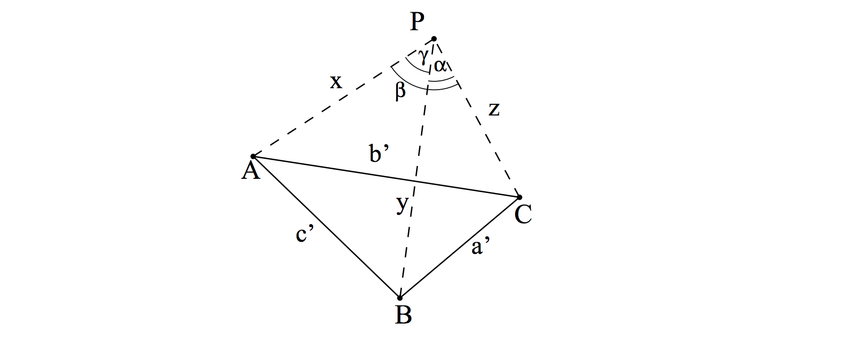
Then the P3P equation system is derived based on the law of cosines (余弦定理):
\[\begin{cases} Y^2 + Z^2 - YZp - a'^2 = 0 \\ Z^2 + X^2 - XZq - b'^2 = 0 \\ X^2 + Y^2 - YXr - c'^2 = 0, \end{cases}\]where \(X\), \(Y\), \(Z\) are variables to be determined.
To simply the equation system, we let \(X= xZ\), \(Y = yZ\), \(c'= \sqrt{v}Z\), \(a'=\sqrt{av}Z\), \(b'=\sqrt{bv}Z\), then the equation system is turned into
\[\begin{cases} y^2 + 1 - py - av = 0 \\ x^2 + 1 - qx -bv = 0 \\ x^2 + y^2 - xyr - v = 0, \end{cases}\]where \(x\), \(y\), \(v\) are variables to be determined.
Eliminating \(v = x^2 + y^2 - xyr\), we have
\[\begin{cases} ax^2 + (a-1)y^2 - ar xy + py =1 \\ (b-1)x^2 + b y^2 - brxy + qx = 1. \end{cases}\]Essentially, the two quatratic equations define two conics, which may have infinite or at most four intersections. Therefore, the P3P problem has either an infinite number of solutions or at most four physical solutions.
P4P, P5P, PnP
Using more than 3 points provides redundant data for the solution of pose estimation. The linear algorithm is generally used [1]. The \(n\) points can form \(\frac{n(n-1)}{2}\) triangles and thus derive \(\frac{n(n-1)}{2}\) second degree polynomial equations based on 余弦定理. By eliminating the set of variables into a single one, we still have \(\frac{n(n-1)}{2} - (n-1) = \frac{(n-1)(n-2)}{2}\) fourth degree polynomial equations. When n = 5, we have the homogeneous equation system:
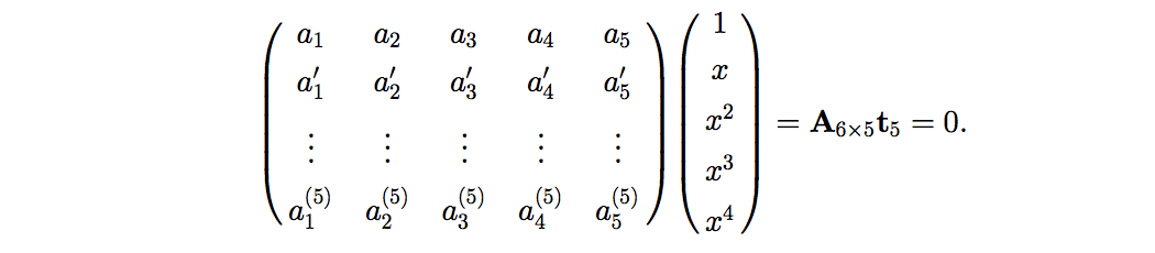
The overdermined equation system can be easily solved by SVD decomposition, where \(t_5\) equals to the right singular vector corresponding to the smallest singular value. The solution can be generalized to cases when \(n>5\).
When \(n=4\), things are a little bit more complicated since the equation system above is underdetermined. We refer the readers to [1] for details.
EPnP
EPnP algorithm is one of the most efficient PnP algorithm which has O(n) complexity. It is composed of three steps:
Step 1. In world coordinate system, find four control points: \(c_j^w (j = 1,...,4)\). One of them is the centroid of the 3D points and the other three are vectors aligned with principle directions of the 3D point set. Then all the 3D points are represented by the barycentric coordinates as a linear combination of the four control points: \(p_i^w = \sum_{j=1}^4 \alpha_{ij} c_j^w (i=1,...,n)\).
Step 2. In camera coordinate system, the equations between 3D points and control points still preserve: \(p_i^c = \sum_{j=1}^4 \alpha_{ij} c_j^c\). Given the 2D projections of the 3D points \(\{p_i\}i=1,...,n\), we have \(\omega_i \begin{bmatrix} u_i \\v_i \\ 1 \end{bmatrix} = K p_i^c = K \sum_{j=1}^4 \alpha_{ij} c_j^c\). Here, \(\omega_i\) and \(\{c_j^c\}j=1,...,4\) are unknowns. By filling in the camera intrinsic matrix, the equation can be expressed as follow:
\[\omega_i \begin{bmatrix} u_i \\ v_i \\ 1 \end{bmatrix} = \begin{bmatrix} f_u & 0 & u_c \\ 0 & f_v & v_c \\ 0 & 0 & 1 \end{bmatrix} \begin{bmatrix} \sum_{j=1}^4 \alpha_{ij} x_j^c \\ \sum_{j=1}^4 \alpha_{ij} y_j^c \\ \sum_{j=1}^4 \alpha_{ij} z_j^c \end{bmatrix}.\]By eliminating \(\omega_i = \sum_{j=1}^4 \alpha_{ij}z_j^c\), we get two linear equations:
\[\begin{cases} \sum_{j=1}^4 \big( \alpha_{ij}f_u x_j^c + \alpha_{ij} (u_c - u_i) z_j^c \big) = 0 \\ \sum_{j=1}^4 \big( \alpha_{ij}f_v y_j^c + \alpha_{ij} (v_c - v_i) z_j^c \big) = 0 \end{cases}.\]Therefore, each 3D-2D correspondence yields two linear equations with respect to a 12-vector \(x=[x_1^c, y_1^c, z_1^c, ..., x_4^c, y_4^c, z_4^c]^T\). If consider all the correspondences, we generate a linear system of the form
\[Mx = 0.\]If we have normalized the coordinates of image pixels to \([u_i, v_i]^T\), the equation system becomes
\[\begin{bmatrix} \alpha_{i1} & \alpha_{i2} & \alpha_{i3} & \alpha_{i4} & 0 & 0 & 0 & 0 & -u_i \alpha_{i1} & -u_i \alpha_{i2} & -u_i \alpha_{i3} & -u_i \alpha_{i4} \\ 0 & 0 & 0 & 0 & \alpha_{i1} & \alpha_{i2} & \alpha_{i3} & \alpha_{i4} & -v_i \alpha_{i1} & -v_i \alpha_{i2} & -v_i \alpha_{i3} & -v_i \alpha_{i4} \end{bmatrix} \begin{bmatrix} x_1^c \\ x_2^c \\ x_3^c \\ x_4^c \\ y_1^c \\ y_2^c \\ y_3^c \\ y_4^c \\ z_1^c \\ z_2^c \\ z_3^c \\ z_4^c \end{bmatrix} \\ = \left(\begin{bmatrix} 1 & 0 & -u_i \\ 0 & 1 & -v_i \end{bmatrix} \otimes \mathbf{\alpha}_i^T \right) \mathbf{x} = \mathbf{0},\]where \(\otimes\) denotes Kronecker product.
Step 3. The solution of the linear equation system lies in the null space or kernel of \(M^TM\) and can be expressed as \(x = \sum_{i=1}^N \beta_i v_i\), where \(v_i\) are the right-singular vectors of \(M\) corresponding to the zero singular values. Now the unknowns become \(\{\beta_i\}i=1,...,N\). Based on the analysis in [2], the dimension \(N\) of null-space of \(M^TM\) varies from 1 to 4. The algorithm then considers all the four cases and choose the best set of \(\{\beta_i\}i=1,...,N\) with the miminum reprojection error.
Other PnPs and insights
- RPnP: A Robust O(n) Solution to the Perspective-n-Point Problem
- OPnP: Revisiting the PnP Problem: A Fast, General and Optimal Solution
- REPPnP: Very Fast Solution to the PnP Problem with Algebraic Outlier Rejection
- ASPnP: ASPnP: An Accurate and Scalable Solution to the Perspective-n-Point Problem
- The accuracy of solutions to the PnP problem is closely related to the configuration of the 3D point set [RPnP]. Ordinary 3D case, planar case, quasisingular case and “uncentered data” [EPnP].
- Under the assumption of independently and identically distribution (i.i.d.) Gaussian noise, minimizing the reprojection error is statistically optimal in the sense of maximum likelihood estimation (MLE).
- Pose ambiguity
Scene COordinate REgression Network (SCORE-Net)
Network architecture
-
Dilated convolution (空洞卷积) Fully convolutional betwork, dilated conv
-
Heteroscedasticity 异方差,变量的方差各不相同。Remidial actions for severe heteroscedasticity are necessary.
-
“Data normalization (or called pre-conditioning in the numerical literature) is an essential step in the DLT algorithm.” from Page 107
-
rank-constrained optimization
-
degenerate cases and the coplanar case
Reference
[1] Linear N-Point Camera Pose Determination
[2] EPnP: An Accurate O(n)Solution to the PnP Problem