Gaussian Process Regression
Gaussian Process
A Gaussian process is a collection of infinite random variables \(\{f(\mathbf{x}): \mathbf{x} \in \mathcal{X} \}\), any finite number of which have a joint Gaussian distribution. It is completely specified by its mean function \(m(\mathbf{x}) = E(f(\mathbf{x}))\) and covariance function \(k(\mathbf{x}, \mathbf{x}') = E( (f(\mathbf{x})-m(\mathbf{x}))(f(\mathbf{x}')-m(\mathbf{x}')) )\).
Consider a simple example of a zero-mean Gaussian process,
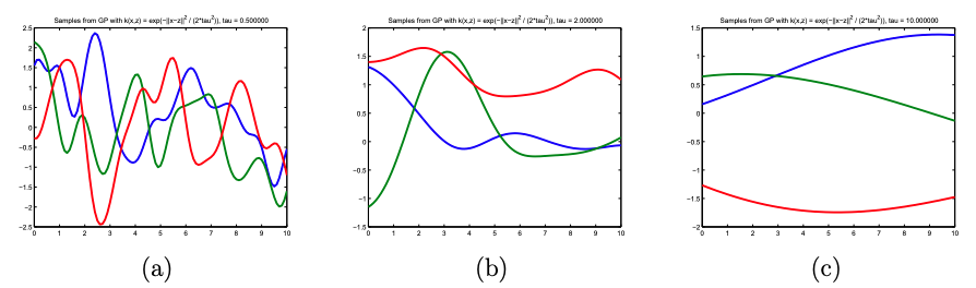
\[f(.) \sim \mathcal{GP}(0, k(.,.)),\]where \(k(x, x') = exp(-\frac{1}{2\tau ^2}\|x-x'\|^2)\) is the squared exponential kernel function. \(f(x)\) and \(f(x')\) will tend to have high covariance (i.e., nearby in output space) if \(x\) and \(x'\) are nearby in the input space, and low covariance in the reverse case. It means that functions drawn from this Gaussian process will tend to be “locally smooth”, as shown in figure below. As the bandwidth parameter \(\tau\) increases (Panel a to b to c), points located far away will have higher correlations, and hence the function tends to be smoother overall.
Gaussian Process Regression (GPR)
Given a set of training data \(D = \{(X,Y)\} = \{(x_i, y_i) \}\), \(i \in [1,n]\), we would like to fit a model to it (\(y=f(x)\)), so that a new output \(y_{n+1}\) can be predicted for the new input set \(X^*\). Sometimes, it is hard to claim \(f(x)\) to some specific models. A Gaussian process is clearly preferable, because it can represent \(f(x)\) obliquely but rigorously by letting the data “speak” for themselves. To make prediction for the new input \(x_{n+1}\) is equivalent to drawing function \(f\) from the posterior distribution \(p(f\|D)\).
For ease of elaboration, we still assume a prior Gaussian process with zero mean for regression. By definition, previous outputs and to-be-determined outputs folow a joint multivariate normal distribution:
\[\begin{bmatrix} Y \\ Y^* \end{bmatrix} ~ N \left(\mathbf{0}, \begin{bmatrix} K(X,X)+\sigma^2 I & K(X, X^*) \\ K(X^*, X) & K(X^*, X^*) \end{bmatrix} \right),\]where \(\sigma\) is the assumed noise level of observations. Then the posterior distribution is a multivariate normal distribution with mean
\[K(X^*, X) [K(X,X) + \sigma^2 I]^{-1} Y\]and covariance Matrix
\[K(X^*, X^*) - K(X^*, X) [K(X,X) + \sigma^2 I]^{-1} Y.\]Thus, the posterior is also a GP with mean function
\[m'(x) = K(x, X) [K(X,X) + \sigma^2 I]^{-1} Y\]and kernel function
\[k'(x, x') = k(x, x') - K(x, X) [K(X,X) + \sigma^2 I]^{-1} K(X, x')\]Interpretation of GPR from the weight view
We can rewrite the posterior mean function as
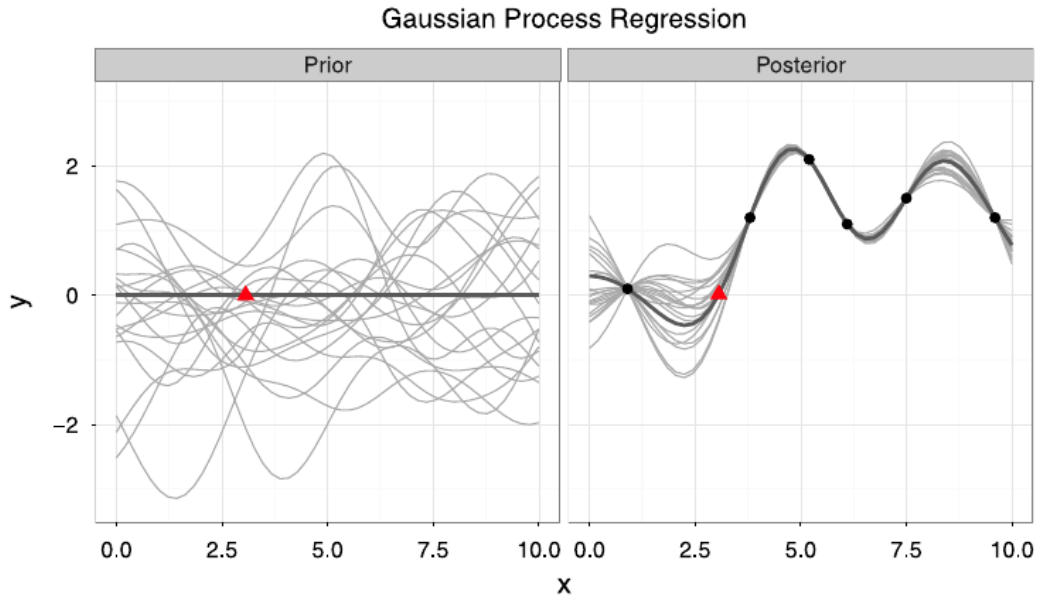
\[m'(x) = \sum_{i=1}^n w_i k(x_i, x),\]where \(x_i \in X\) is previously observed and \(w_i \in w = [K(X,X) + \sigma^2 I]^{-1} Y\). This equation shows that Gaussian process regression is equivalent to a linear regression model using basis functions \(k\) to project the input into a feature space. To make new predictions, every output \(y_i\) is weighted by how similar its associated input \(x_i\) is to the to-be-predicted point \(x\) by a similarity measure induced by the kernel \(k(x_i, x)\). In figure below, Panel left shows a set of Gaussian process drawn from the prior and Panel right shows Gaussian processes drawn from the posterior with observations marked by the dots. The mean function is marked in dark grey.
Reference
Gaussian Processes for Dummies
Gaussian Processes for Machine Learning (MIT)